03 - Receptive Fields in Depth

Computing Receptive Fields of CNNs

Attribution

This note is adapted from:
André Araujo, Wade Norris, Jack Sim, “Computing Receptive Fields of Convolutional Neural Networks”, Distill (2019).
DOI: 10.23915/distill.00021 — https://distill.pub/2019/computing-receptive-fields
Licensed under CC-BY 4.0.
Changes: restructuring into Markdown format, addition of custom explanations/examples.

---

Overview

The following discussion focuses on fully-convolutional neural networks (CNNs), deriving both the size of the receptive field and the position of output feature receptive fields relative to the input signal.

Note

The derivations are broad enough to apply to any type of input signal to convolutional neural networks, though images are used as the recurring example, with references to modern computer vision architectures where appropriate.

Road Map

First:

• Closed-form expressions are derived for the case where the network has a single path from input to output (as in AlexNet or VGG).

Next:

• The more general case of arbitrary computation graphs with multiple paths from input to output (as in ResNet or Inception) is discussed.

Last

• Potential alignment issues that may arise in this setting are then considered, and an algorithm is presented to compute the receptive field size and locations.

---

Problem setup

Let’s consider a fully-convolutional neural network (CNN) with $L$ layers, $l=1,2,\dots ,L$.
In addition:

• The feature map $f_l\in {\mathbb{R}}^{h_l\times w_l\times d_l}$ is defined as the output of the $l$-th layer, with height $h_l$, width $w_l$, and depth $d_l$.
• The input image is denoted by $f_0$.
• The final output feature map corresponds to $f_L$.

Focus on $1D$ case

For simplicity, the following analysis focuses on the dimensions along a single axis (e.g., height or width) by considering $1$-dimensional input signals and feature maps. For higher-dimensional signals (e.g., $2D$ images), the derivations can be applied to each dimension independently. Similarly, the figures depict $1$-dimensional depth, since this does not affect the receptive field computation.

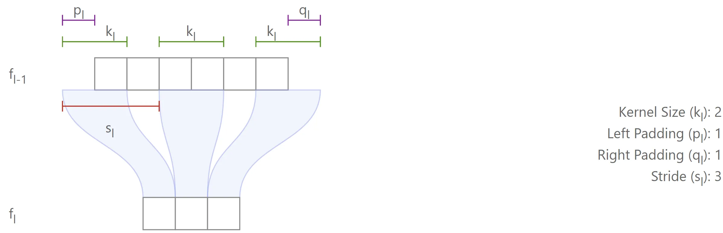
The spatial configuration of each layer $l$ is parameterized by four variables, as illustrated in the figure below:

• $k_l$: kernel size (positive integer)
• $s_l$: stride (positive integer)
• $p_l$: padding applied to the left side of the input feature map (non-negative integer).¹
• $q_l$: padding applied to the right side of the input feature map (non-negative integer)

Note

Only layers whose output features depend locally on input features are considered: e.g., convolution, pooling, or elementwise operations such as non-linearities, addition and filter concatenation. These are commonly used in state-of-the-art networks. Elementwise operations are defined to have a “kernel size” of $1$, since each output feature depends on a single location of the input feature maps.

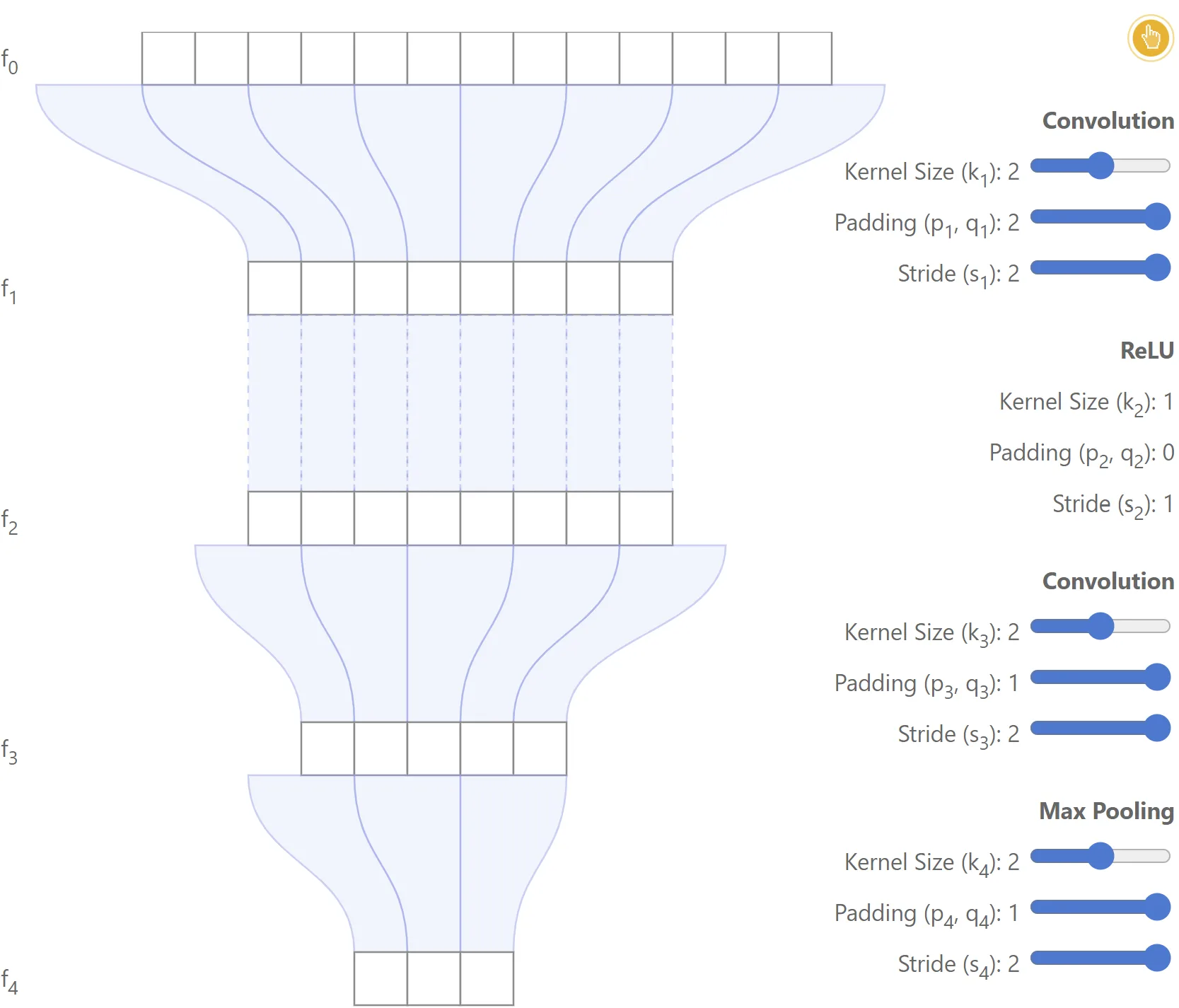
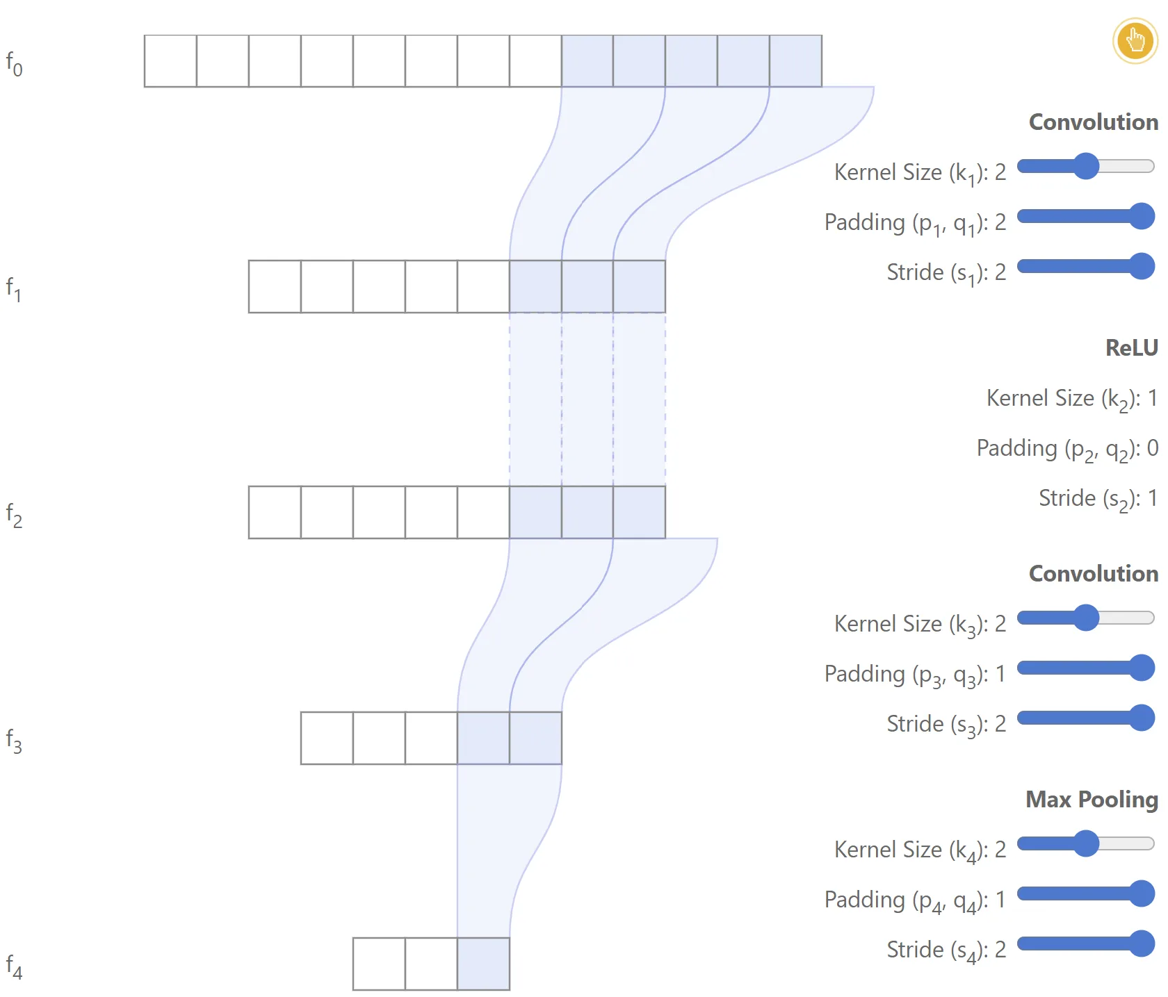
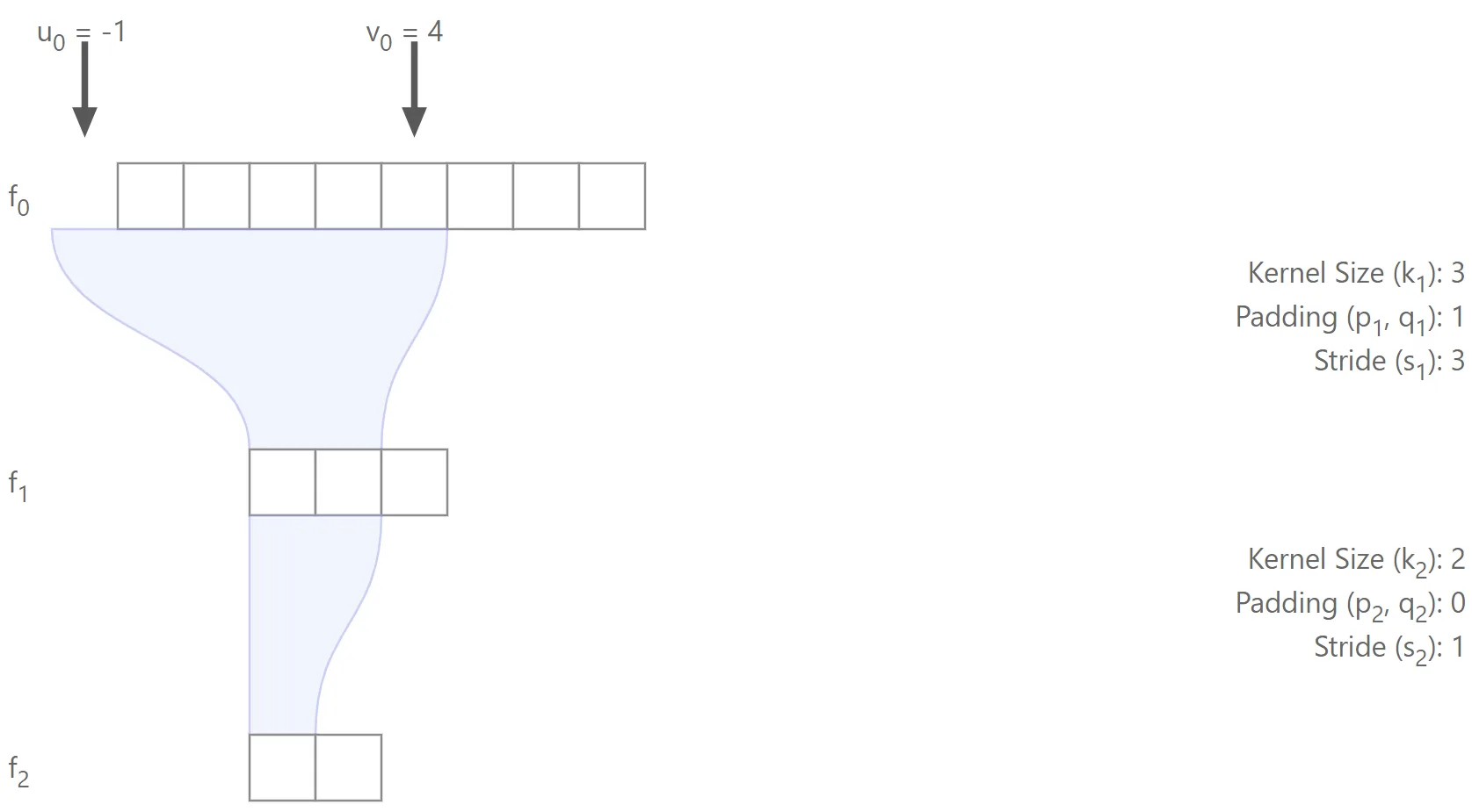
The notation is further illustrated with the simple network shown below.

Example

In this case, $L=4$, and the model consists of a convolutional layer, followed by a ReLU, a second convolutional layer, and a max-pooling operation.²

---

Single-path networks

In this section, recurrence and closed-form expressions are computed for fully convolutional networks with a single path from input to output (e.g., AlexNet or VGG).

Computing receptive field size

Definition of $r_l$

$r_l$ is defined as the size of the receptive field of the final output feature map $f_L$ with respect to the feature map $f_l$.
In other words, $r_l$ corresponds to the number of features in the feature map $f_l$ which contribute to generate a single feature in $f_L$. Note that $r_L=1$.

Example

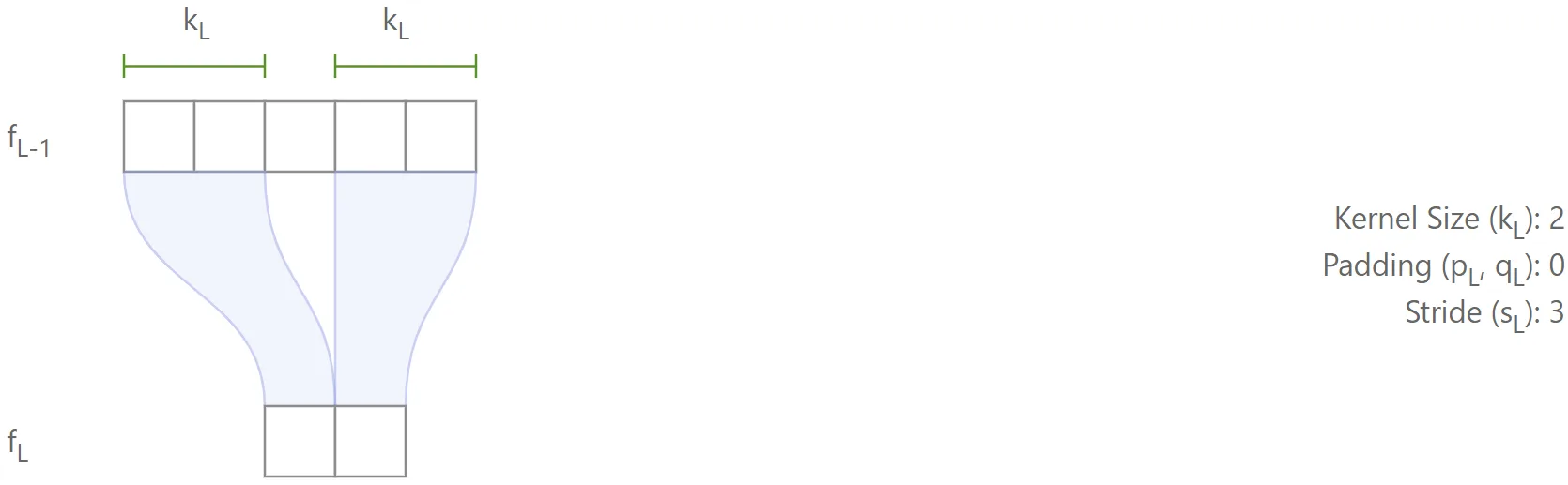
As a simple example, let’s consider layer $L$, which takes the features $f_{L-1}$ as input and produces $f_L$ as output. An illustration is shown below:

It is easy to see that $k_L$ features of $f_{L-1}$ can influence a single feature of $f_L$, since each feature of $f_L$ is directly connected to $k_L$ features of $f_{L-1}$. Consequently, $r_{L-1}=k_L$.

Computing $r_{l-1}$ given $r_l$

Let’s consider now the more general case where $r_l$ is known and $r_{l-1}$ is to be computed. Each feature of $f_l$ is connected to $k_l$ features of $f_{l-1}$

Case $k_l=1$

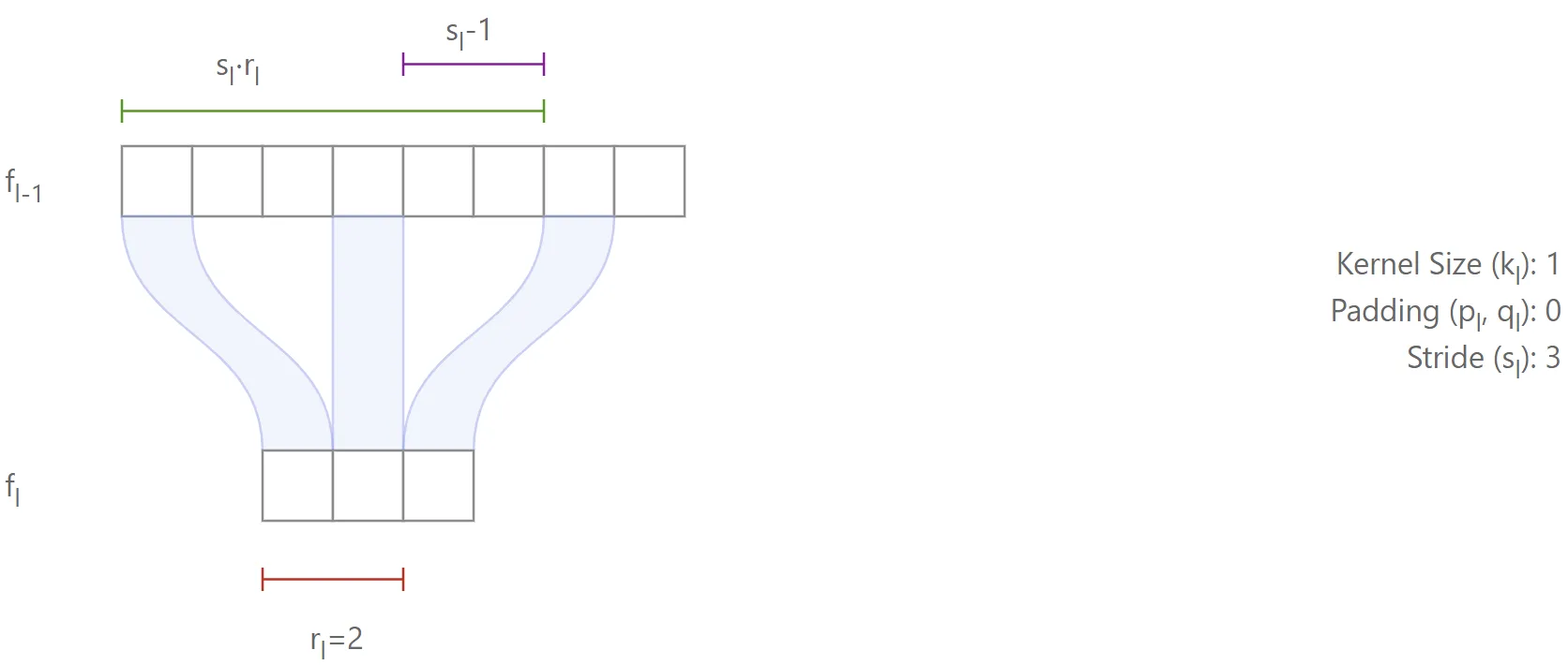
First, consider the situation where $k_l=1$: in this case, the $r_l$ features in $f_l$ will cover

$$r_{l-1}=s_l\cdot r_l-(s_l-1)$$

features in $f_{l-1}$.

This is illustrated in the figure below, where $r_l=2$ (highlighted in red).
The first term $s_l\cdot r_l$ (in green) covers the entire region from which the features originate, but it also covers $s_l-1$ excess features (in purple), which must therefore be subtracted.³

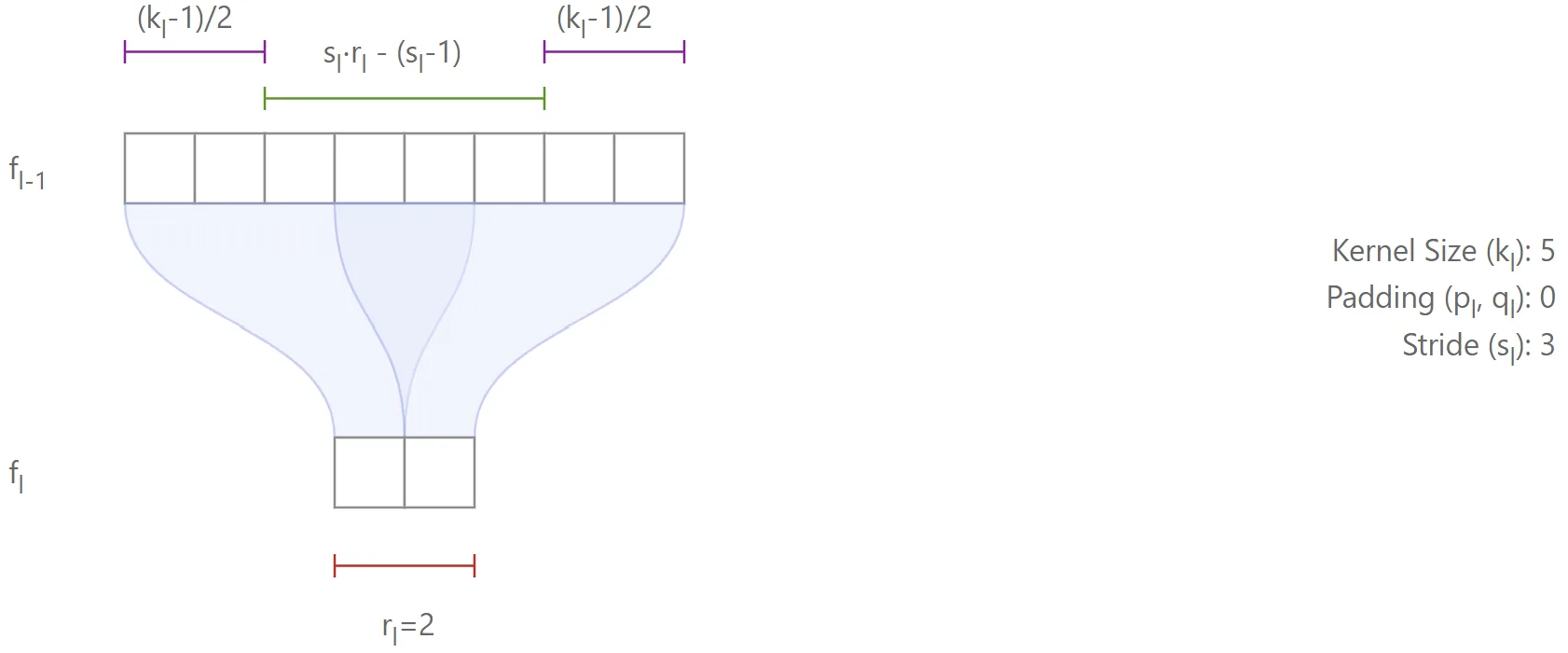
Case $k_l>1$

When $k_l>1$, the receptive field expands by $k_l-1$ additional features, which will cover those from the left and the right of the region. For example:

• With a kernel size of 5 ($k_l=5$), there are 2 extra features on each side, for a total of 4.
• With a kernel size of 4 ($k_l=4$), the distribution is not symmetric (e.g., 1 feature on the left and 2 on the right), but the total number of additional features is still $k_l-1=3$.

Thus, whether $k_l$ is odd or even, the left and right extensions always add up to $k_l-1$ in total.⁴

This yields the general recursive equation (first-order, non-homogeneous, with variable coefficients):

$$\boxed{r_{l-1}=s_l\cdot r_l+(k_l-s_l)}\text{\hspace{1em}(1)}$$

This equation can be used in a recursive algorithm to compute the receptive field size of the network, $r_0$. However, more can be done: the recursive equation can in fact be solved to obtain an explicit solution as a function of the values of $k_l$ and $s_l$:

$$\boxed{r_0=\sum _{l=1}^L\left((k_l-1)\cdot \prod _{i=1}^{l-1}{s}_i\right)+1}\text{\hspace{1em}(2)}$$

This expression has an intuitive meaning, as can be seen by considering a few special cases. For example:

• if all kernels have size $1$, the receptive field will naturally also have size 1.
• if all strides are equal to $1$, then the receptive field is simply the sum of $(k_l-1)$ across all layers, plus $1$, which is easy to verify.
• if instead the stride is greater than $1$ for a particular layer, the receptive field increases proportionally for all lower layers.

Proof of the formula for the receptive field size

The first trick to solve (1) is to multiply it by ${\prod }_{i=1}^{l-1}{s}_i$:

$$r_{l-1}\prod _{i=1}^{l-1}{s}_i=s_l\cdot r_l\prod _{i=1}^{l-1}{s}_i+(k_l-s_l)\prod _{i=1}^{l-1}{s}_i=r_l\prod _{i=1}^l{s}_i+k_l\prod _{i=1}^{l-1}{s}_i-\prod _{i=1}^l{s}_i\text{\hspace{1em}(14)}$$

Define $A_l=r_l{\prod }_{i=1}^l{s}_i$, and note that ${\prod }_{i=1}^0{s}_i=1$ (since $1$ is the neutral element for multiplication), so $A_0=r_0$. Using this definition, (14) can be rewritten as:

$$A_l-A_{l-1}=\prod _{i=1}^l{s}_i-k_l\prod _{i=1}^{l-1}{s}_i\text{\hspace{1em}(15)}$$

Now, summing from $l=1$ to $l=L$:

$$\sum _{l=1}^L(A_l-A_{l-1})=A_L-A_0=\sum _{l=1}^L(\prod _{i=1}^l{s}_i-k_l\prod _{i=1}^{l-1}{s}_i)\text{\hspace{1em}(16)}$$

Note that $A_0=r_0$ and $A_L=r_L{\prod }_{i=1}^L{s}_i={\prod }_{i=1}^L{s}_i$. Therefore, it’s possible to compute:

$$\begin{array}{rl}{r}_0& =\prod _{i=1}^L{s}_i+\sum _{l=1}^L(k_l\prod _{i=1}^{l-1}{s}_i-\prod _{i=1}^l{s}_i)\\ & =\sum _{l=1}^L{k}_l\prod _{i=1}^{l-1}{s}_i-\sum _{l=1}^{L-1}\prod _{i=1}^l{s}_i\\ & =\sum _{l=1}^L{k}_l\prod _{i=1}^{l-1}{s}_i-\sum _{l=1}^L\prod _{i=1}^{l-1}{s}_i+1\end{array}\text{\hspace{1em}(17)}$$

where the last step is done by a change of variables for the right term.

Finally, rewriting (17), we obtain the expression for the receptive field size $r_0$ of a CNN on the input image, given the parameters of each layer:

$$r_0=\sum _{l=1}^L((k_l-1)\prod _{i=1}^{l-1}{s}_i)+1\text{\hspace{1em}(18)}$$

Note

Finally, note that padding does not need to be taken into account in this derivation.

Padding only introduces artificial cells (e.g., zeros) at the borders of the input, which may be included in the receptive field of boundary features.
However, it does not change the receptive field size, since this is determined exclusively by kernel sizes and strides.
In other words, padding affects which pixels are used at the borders, but not how many input positions are covered in total.

---

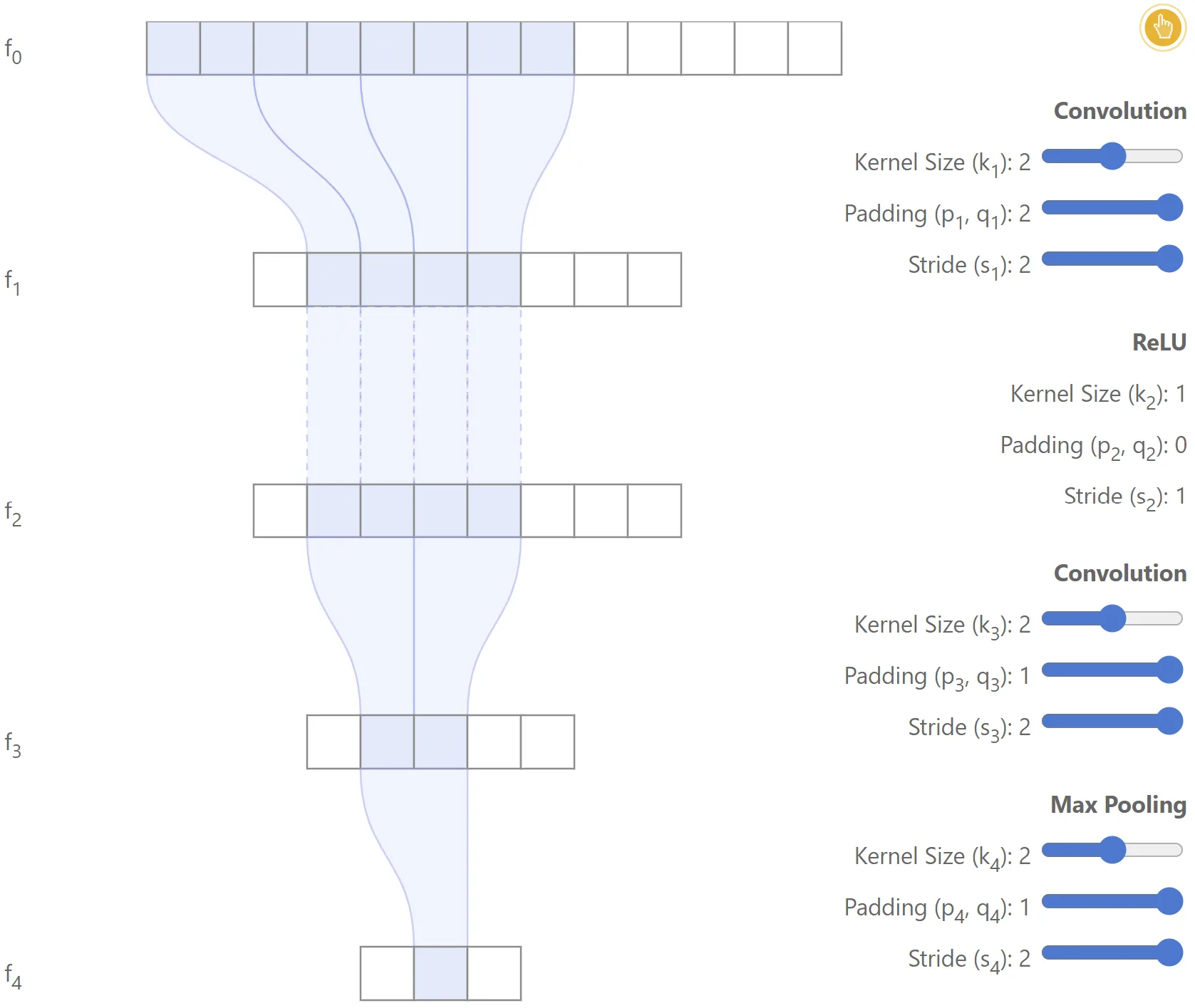
Computing receptive field region in input image

While it is important to know the size of the region that generates one feature in the output feature map, in many cases it is also critical to precisely localize the region that generated a feature.

Question

For example, given feature $f_L(i,j)$, what is the region in the input image that generated it?

This is addressed in this section.

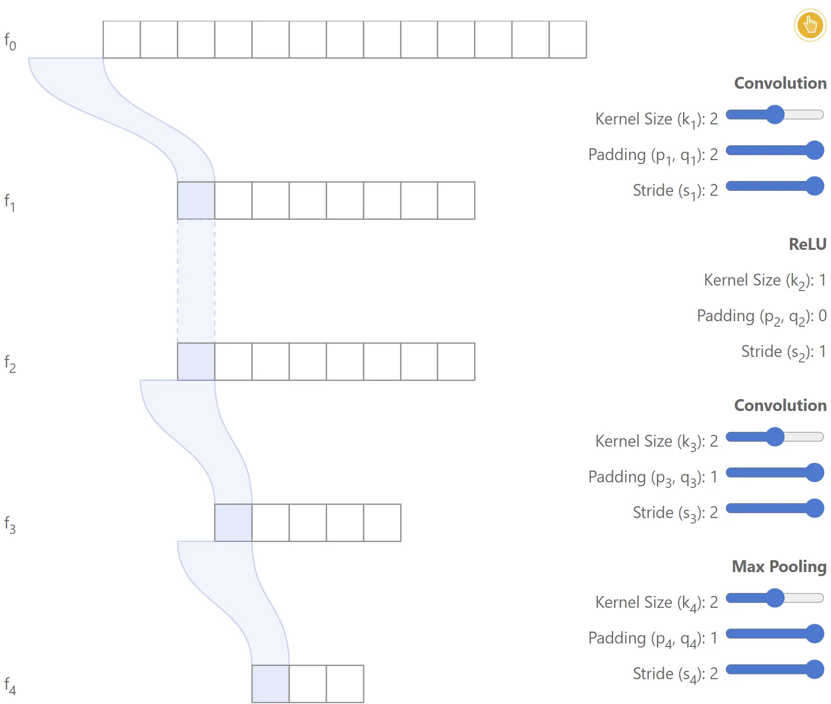
Let’s denote $u_l$ and $v_l$ the left-most and right-most coordinates (in $f_l$) of the region used to compute the desired feature in $f_L$.

Note

In these derivations, the coordinates are zero-indexed (i.e., the first feature in each map is at coordinate $0$).
Note that $u_L=v_L$ corresponds to the location of the desired feature in $f_L$.

Example

The figure below illustrates a simple 2-layer network, where it’s highlighted the region in $f_0$ used to compute the first feature from $f_2$.
Note that in this case the region includes some padding.

In this example:

• $u_2=v_2=0$
• $u_1=0$, $v_1=1$
• $u_0=-1$, $v_0=4$
  
  

Question

Let’s begin by asking: given $u_l,v_l$, is it possible to compute $u_{l-1},v_{l-1}$?

Consider the simple case where $u_l=0$ (this corresponds to the first position in $f_l$). In this case, the left-most feature $u_{l-1}$ will clearly be located at $-p_l$, since the first feature will be generated by placing the left end of the kernel over that position.

If $u_l=1$ (the second feature), the left-most position is $u_{l-1}=-p_l+s_l$ ; for $u_l=2$, one obtains $u_{l-1}=-p_l+2\cdot s_l$, and so on. In general:

$$\begin{array}{rl}{u}_{l-1}& =-p_l+u_l\cdot s_l\\ v_{l-1}& =-p_l+v_l\cdot s_l+k_l-1\end{array}\text{\hspace{1em}(3)(4)}$$

where the computation of $v_{l-1}$ differs only by the addition of $k_l-1$, which is needed since in this case we want to find the right-most position.

Note that these expressions are very similar to the recursion derived for the receptive field size $(1)$. As before, one could implement a recursion over the network to obtain $u_l,v_l$ for each layer; however, one can also solve directly for $u_0,v_0$ and obtain closed-form expressions in terms of the network parameters:

$$\boxed{u_0=u_L\prod _{i=1}^L{s}_i-\sum _{l=1}^L{p}_l\prod _{i=1}^{l-1}{s}_i}\text{\hspace{1em}(5)}$$

Solving the recursive equations: receptive field region

The derivations are analogous to those used to solve (1).
Let’s consider the computation of $u_0$. First, multiply (3) by ${\prod }_{i=1}^{l-1}{s}_i$:

$$u_{l-1}\prod _{i=1}^{l-1}{s}_i=u_l\cdot s_l\prod _{i=1}^{l-1}{s}_i-p_l\prod _{i=1}^{l-1}{s}_i=u_l\prod _{i=1}^l{s}_i-p_l\prod _{i=1}^{l-1}{s}_i\text{\hspace{1em}(19)}$$

Define $B_l=u_l{\prod }_{i=1}^l{s}_i$, and rewrite (19) as:

$$B_l-B_{l-1}=p_l\prod _{i=1}^{l-1}{s}_i\text{\hspace{1em}(20)}$$

Summing from $l=1$ to $l=L$:

$$\sum _{l=1}^L(B_l-B_{l-1})=B_L-B_0=\sum _{l=1}^L{p}_l\prod _{i=1}^{l-1}{s}_i\text{\hspace{1em}(21)}$$

Note that $B_0=u_0$ and $B_L=u_L{\prod }_{i=1}^L{s}_i$. Therefore:

$$u_0=u_L\prod _{i=1}^L{s}_i-\sum _{l=1}^L{p}_l\prod _{i=1}^{l-1}{s}_i\text{\hspace{1em}(22)}$$

This yields the left-most feature position in the input image as a function of the padding $(p_l)$ and stride $(s_l)$ applied in each layer of the network, and of the feature location in the output feature map $(u_L)$.

And for the right-most feature location $v_0$:

$$\boxed{v_0=v_L\prod _{i=1}^L{s}_i-\sum _{l=1}^L\left(1+p_l-k_l\right)\prod _{i=1}^{l-1}{s}_i}\text{\hspace{1em}(6)}$$

Note

Note that, unlike (5), this expression also depends on the kernel sizes $k_l$ of each layer.

Relation between receptive field size and region

It may be observed that the receptive field size $r_0$ should be directly related to and . Indeed, it is straightforward to show that $r_0=v_0-u_0+1$. In particular, this implies that $(6)$ can be rewritten as:

$$\boxed{v_0=u_0+r_0-1}\text{\hspace{1em}(7)}$$

Effective stride and padding

To compute $u_0$ and $v_0$ in practice, it is convenient to define two variables that depend only on the paddings and strides of the different layers:

• Effective stride:

$$S_l=\prod _{i=l+1}^L{s}_i$$

represents the stride between a given feature map $f_l$ and the output feature map $f_L$.

• Effective padding:

$$P_l=\sum _{m=l+1}^L{p}_m\prod _{i=l+1}^{m-1}{s}_i$$

represents the padding between a given feature map $f_l$ and the output feature map $f_L$.

With these definitions, equation $(5)$ can be rewritten as:

$$u_0=-P_0+u_L\cdot S_0\text{\hspace{1em}(8)}$$

Note the resemblance between $(8)$ and $(3)$. By using $S_l$ and $P_l$, one can compute the locations $u_l,v_l$ for the feature map $f_l$ given the location at the output feature map $u_L$.

When computing feature locations for a given network, it is useful to precompute three variables: $P_0,S_0,r_0$. Using these three, $u_0$ is obtained from $(8)$ and $v_0$ from $(7)$. This yields the mapping from any output feature location to the input region which influences it.

It is also possible to derive recurrence equations for the effective stride and effective padding. It is straightforward to show that:

$$\begin{array}{rl}{S}_{l-1}& =s_l\cdot S_l\\ P_{l-1}& =s_l\cdot P_l+p_l\end{array}\text{\hspace{1em}(9)(10)}$$

These expressions will be handy when deriving an algorithm to solve the case for arbitrary computation graphs, presented in the next section.

Center of receptive field region

Important

It is also interesting to derive an expression for the center of the receptive field region which influences a particular output feature.

This can be used as the location of the feature in the input image

Let’s define the center of the receptive field region for each layer as:

$$c_l=\frac{u_l+v_l}{2}$$

Given the above expressions for $u_0$, $v_0$, and $r_0$, $c_0$ follows immediately (recalling that $u_L=v_L$):

$$\begin{array}{rl}{c}_0& =u_L\prod _{i=1}^L{s}_i-\sum _{l=1}^L\left(p_l-\frac{k_l-1}{2}\right)\prod _{i=1}^{l-1}{s}_i\\ & =u_L\cdot S_0-\sum _{l=1}^L\left(p_l-\frac{k_l-1}{2}\right)\prod _{i=1}^{l-1}{s}_i\\ & =-P_0+u_L\cdot S_0+\frac{r_0-1}{2}\end{array}\text{\hspace{1em}(11)}$$

This expression can be compared to $(8)$ to observe that the center is shifted from the left-most pixel by $\frac{r_0-1}{2}$, which makes sense. Note that the centers of the receptive fields for different output features are spaced by the effective stride $S_0$, as expected.

It is also worth noting that if $p_l=\frac{k_l-1}{2}$ for all layers $l$, the centers of the receptive field regions for the output features will be aligned to the first pixel of the image and located at:

$$0,S_0,2S_0,3S_0,\dots$$

(in this case all $k_l$ must be odd).

Other network operations

Dilated (atrous) convolution

Dilations introduce “holes” in a convolutional kernel. While the number of weights is unchanged, they are no longer applied to spatially adjacent samples. Dilating a kernel by a factor $\alpha$ introduces a stride of $\alpha$ between the sampled positions. Thus, the spatial span of a kernel of size $k>0$ becomes $\alpha (k-1)+1$. The derivations above can be reused by replacing $k$ with $\alpha (k-1)+1$ for any layer that uses dilation.

Upsampling

Often implemented via interpolation (e.g., bilinear, bicubic, nearest neighbor), which yields an equal or larger receptive field since each output depends on one or more input features. For receptive-field computations, treat an upsampling layer as having an effective kernel size equal to the number of input features used to produce one output feature.

Separable convolutions

Convolutions separable in spatial or channel dimensions have the same receptive-field properties as their equivalent non-separable convolutions. For example, a $3\times 3$ depth-wise separable convolution has an effective kernel size of $3$ for receptive-field computation.

Batch normalization

At inference time, batch normalization is a feature-wise operation and does not alter the network’s receptive field. During training, however, its parameters are computed from all activations of a layer, so its receptive field is the entire input image.

---

Arbitrary computation graphs

Most state-of-the-art convolutional neural networks (e.g., ResNet and Inception) rely on models where each layer may have more than one input, which means that there might be several different paths from the input image to the final output feature map. These architectures are usually represented using directed acyclic computation graphs, where the set of nodes $N$ represents the layers and the set of edges $E$ encodes the connections between them (feature maps flow through the edges).

The computation presented in the previous section can be used for each of the possible paths from input to output independently. The situation becomes trickier when one wants to take into account all different paths to find the receptive field size of the network and the receptive field regions which correspond to each of the output features.

Alignment issues

Danger

The first potential issue is that one output feature may be computed using misaligned regions of the input image, depending on the path from input to output. Also, the relative position between the image regions used for the computation of each output feature may vary.

As a consequence, the receptive field size may not be shift-invariant.

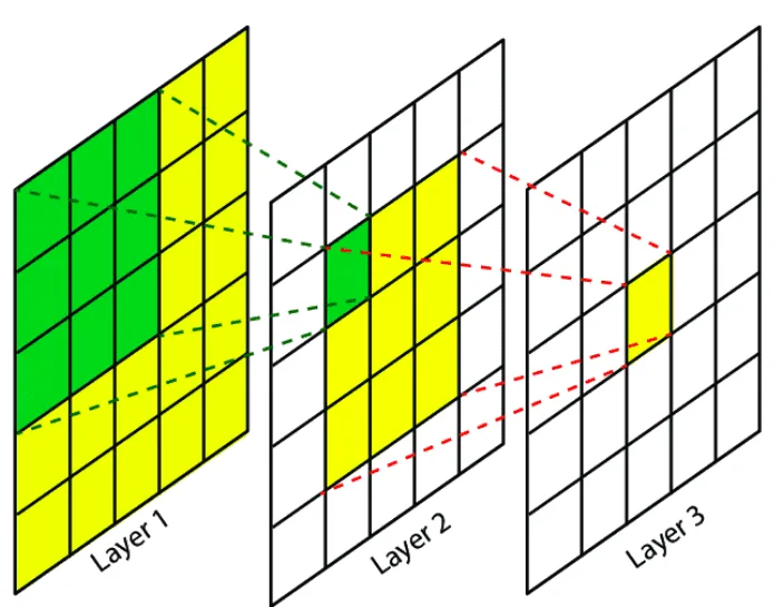
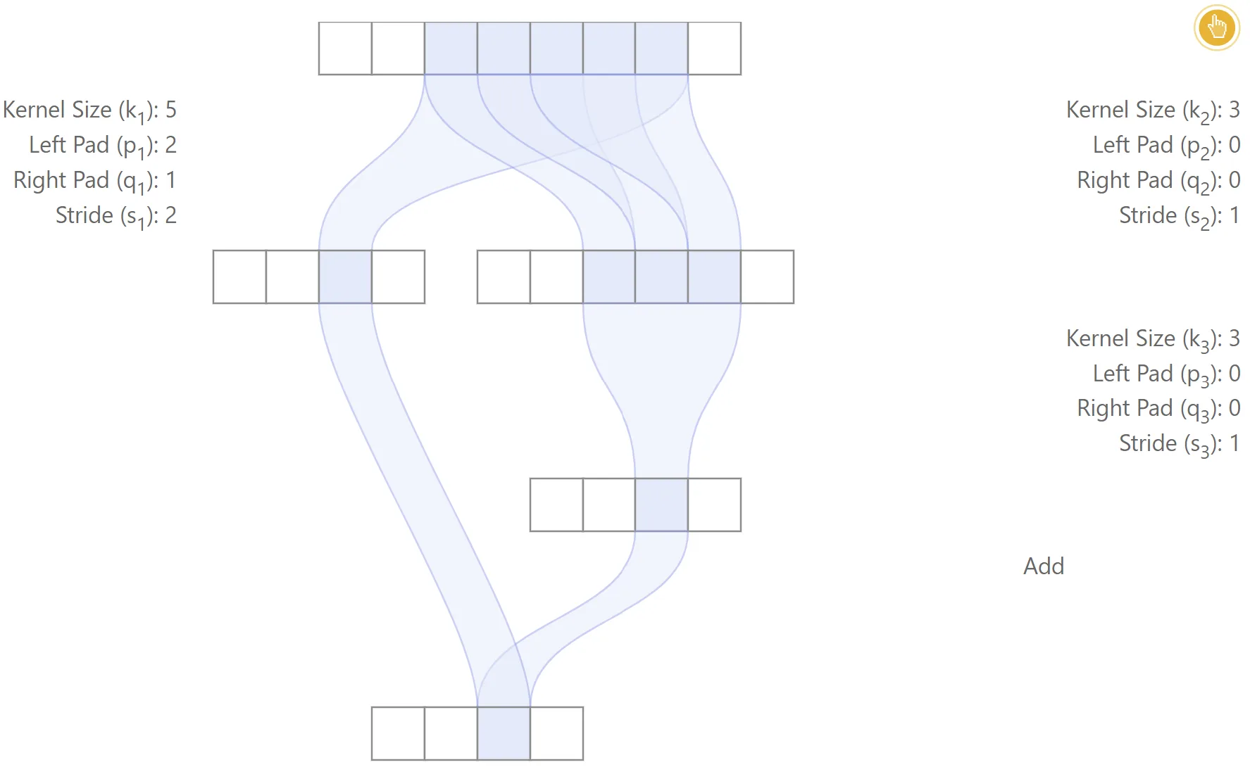
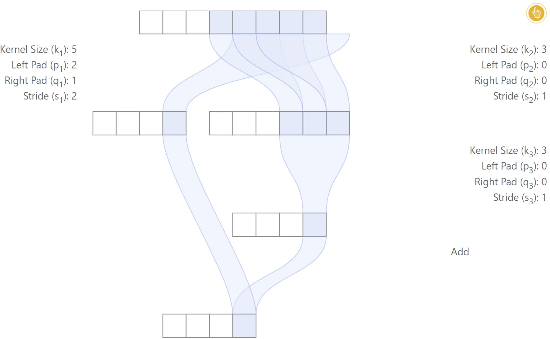
This is illustrated in the figure below with a toy example, in which case the centers of the regions used in the input image are different for the two paths from input to output.

Misaligned network

In this example, padding is used only for the left branch. The first three layers are convolutional, while the last layer performs a simple addition. The relative position between the receptive field regions of the left and right paths is inconsistent for different output features, which leads to a lack of alignment

Also, note that the receptive field size for each output feature may be different. For the second output feature from the left, $6$ input samples are used, while only $5$ are used for the third output feature. This means that the receptive field size may not be shift-invariant when the network is not aligned.

Note

For many computer vision tasks, it is highly desirable that output features be aligned: “image-to-image translation” tasks (e.g., semantic segmentation, edge detection, surface normal estimation, colorization, etc), local feature matching and retrieval, among others.

Important

When the network is aligned, all different paths lead to output features being centered consistently in the same locations. All different paths must have the same effective stride. It is easy to see that the receptive field size will be the largest receptive field among all possible paths. Also, the effective padding of the network corresponds to the effective padding for the path with largest receptive field size, such that one can apply $(8)$ , $(11)$ to localize the region which generated an output feature.

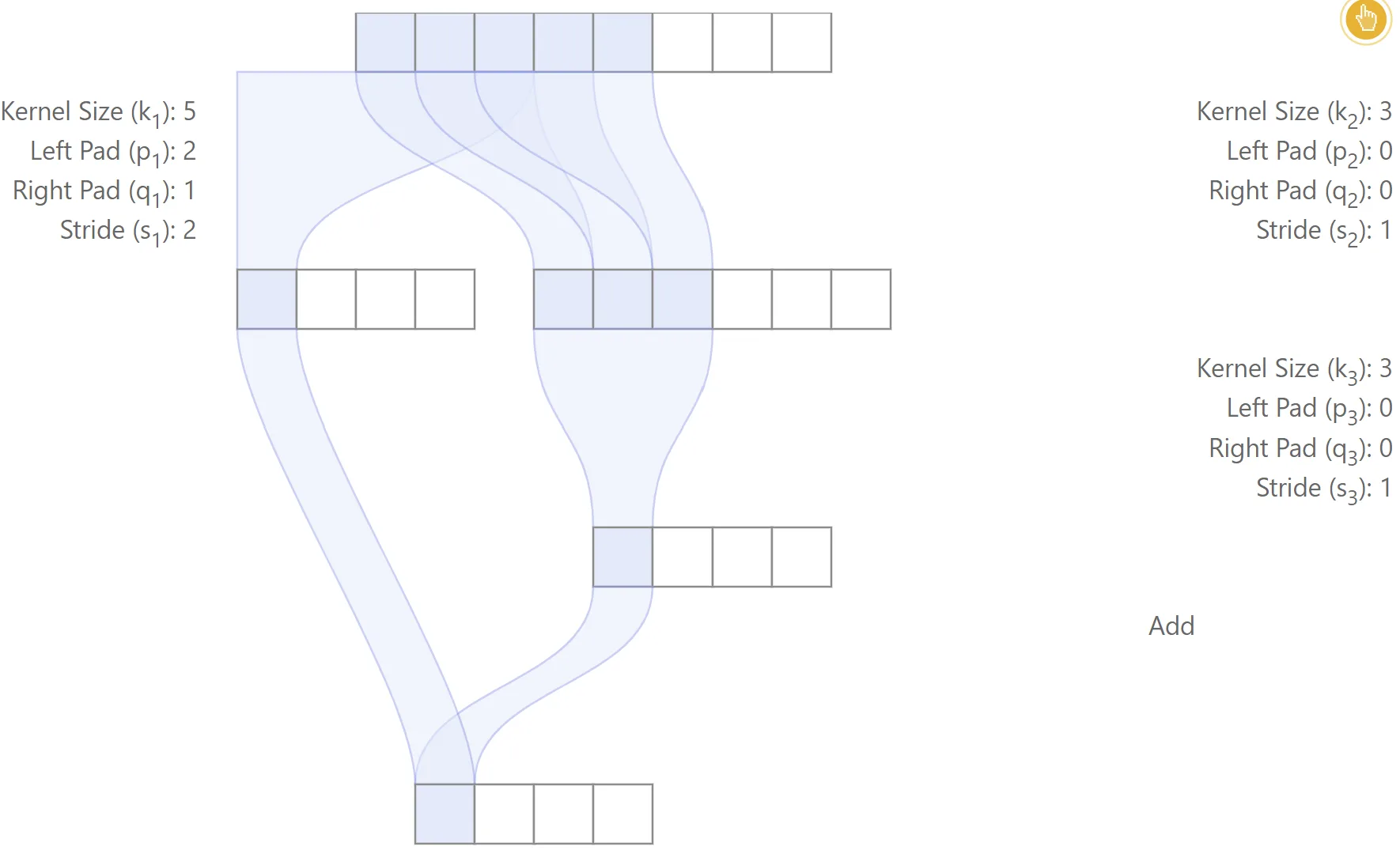
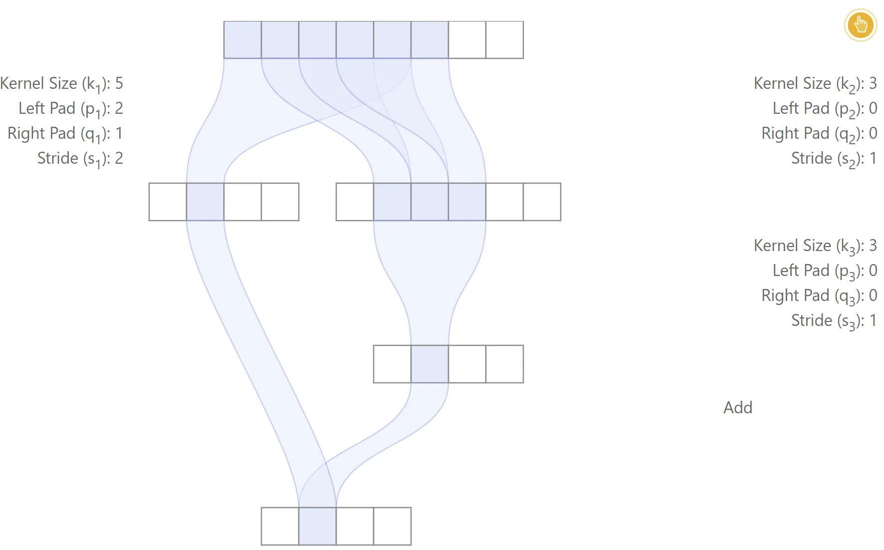
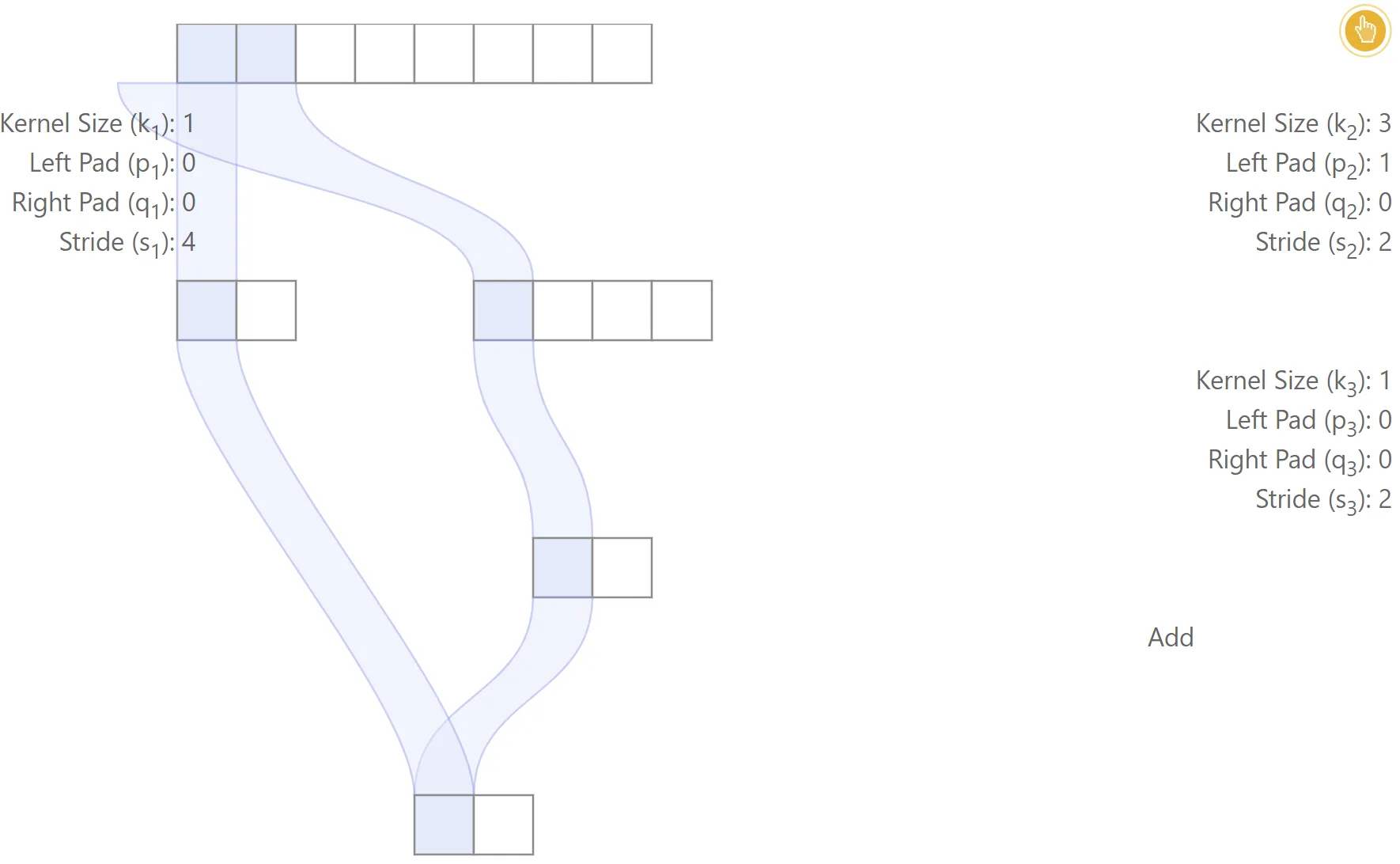
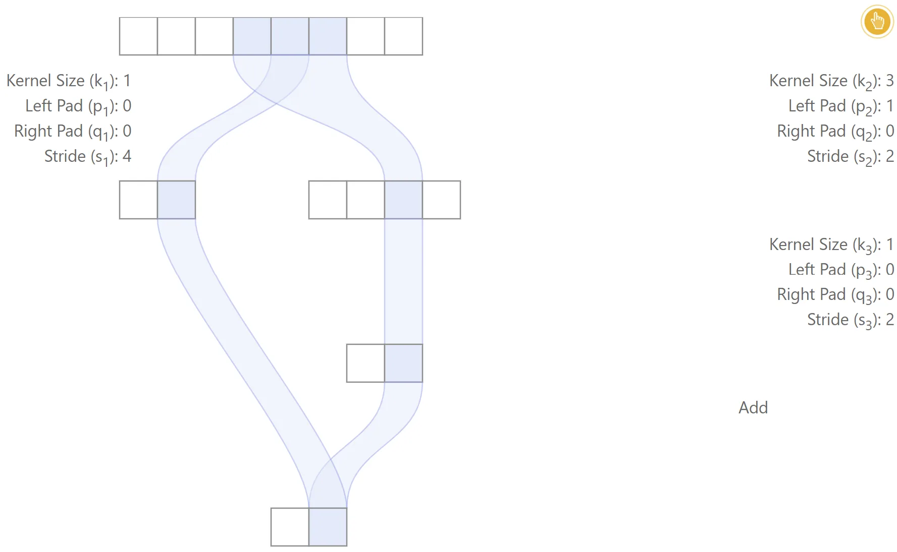
Aligned network

The figure below gives one simple example of an aligned network. In this case, the two different paths lead to each output feature being centered at the same locations. The receptive field size is $3$, the effective stride is $4$ and the effective padding is $1$.

Alignment criteria

More precisely, for a network to be aligned at every layer, we need every possible pair of paths $i$ and $j$ to have $c_l^{(i)}=c_l^{(j)}$ for any layer $l$ and output feature $u_L$. For this to happen, we can see from $(11)$ that two conditions must be satisfied:

$$S_l^{(i)}=S_l^{(j)}\text{\hspace{1em}(12)}$$ $$-P_l^{(i)}+\left(\frac{r_l^{(i)}-1}{2}\right)=-P_l^{(j)}+\left(\frac{r_l^{(j)}-1}{2}\right)\text{\hspace{1em}(13)}$$

for all $i$, $j$, $l$.

Footnotes

1. A more general definition of padding can also be considered: negative padding, interpreted as cropping, can be used in the following derivations without any modification. To keep the presentation concise, the discussion focuses exclusively on non-negative padding. ↩

2. The first output feature of each layer is computed by placing the kernel at the left-most position of the input, including padding, This convention is used by all major Deep Learning libraries. ↩

3. As shown in the illustration below, in some cases the receptive field region may contain “holes”, meaning that some of the input features may be unused for a given layer. ↩

4. Due to border effects, note that the size of the region in the original image which is used to compute each output feature may be different. This happens if padding is used, in which case the receptive field for border features includes the padded region. Later in the article, we discuss how to compute the receptive field region for each feature, which can be used to determine exactly which image pixels are used for each output feature. ↩