Discrete Convolution

In the previous example with the thermometer, the assumption of having a measurement available at every instant is not realistic. In practice, when working with data on a computer, time is discretized, and the sensor provides data at regular intervals. A more realistic assumption is that the thermometer produces one measurement per second. The time index $t$ can then take only integer values. Under the assumption that both $x$ and $w$ are defined only for integer $t$, the discrete convolution can be introduced:

$$s(t)=(x\ast w)(t)=\sum _{a=-\infty }^{\infty }x(a)w(t-a)$$

Note

Since each element of the input and kernel must be explicitly stored separately, it is usually assumed that these functions are zero everywhere except for the finite set of points at which values are stored. This implies that, in practice, the infinite summation described above can be implemented as a summation over a finite number of array elements.

Info

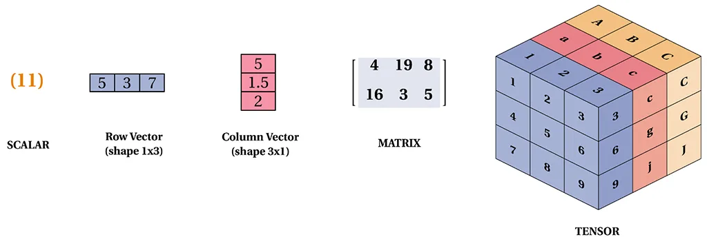
In Machine Learning applications, the input is typically a multidimensional array of data, and the kernel is a multidimensional array of parameters that are adapted by the learning algorithm. Such multidimensional arrays are referred to as tensors.

---

2D Discrete Convolution

Convolutions are often applied along more than one axis at a time. For example, if a two-dimensional image $I$ is used as input, it is natural to employ a two-dimensional kernel $K$ as well:

$$\mathbf{S}(i,j)=(\mathbf{I}\ast \mathbf{K})(i,j)=\sum _m\sum _n\mathbf{I}(m,n)\mathbf{K}(i-m,j-n)\text{\hspace{1em}(1)}$$

Convolution is commutative, which means that it can equivalently be written as:

$$\mathbf{S}(i,j)=(\mathbf{K}\ast \mathbf{I})(i,j)=\sum _m\sum _n\mathbf{I}(i-m,j-n)\mathbf{K}(m,n)\text{\hspace{1em}(2)}$$

Proof

Definition. For two arrays/functions $I$ and $K$:

$$(\mathbf{I}\ast \mathbf{K})(i,j)=\sum _m\sum _n\mathbf{I}(m,n)\mathbf{K}(i-m,j-n).$$

Step 1. Compute $\mathbf{K}\ast \mathbf{I}$.

$$(\mathbf{K}\ast \mathbf{I})(i,j)=\sum _m\sum _n\mathbf{K}(m,n)\mathbf{I}(i-m,j-n).$$

Step 2. Change variables.
Let $u=i-m$, $v=j-n$ , so

$$\begin{gathered} m=i-u \\ n=j-v \end{gathered}$$

Substituting:

$$(\mathbf{K}\ast \mathbf{I})(i,j)=\sum _u\sum _v\mathbf{K}(i-u,j-v)\mathbf{I}(u,v).$$

Step 3. Reorder terms.

$$(\mathbf{K}\ast \mathbf{I})(i,j)=\sum _u\sum _v\mathbf{I}(u,v)\mathbf{K}(i-u,j-v).$$

Step 4. Rename dummy indices.
The summation indices $u,v$ are dummy variables: they can be renamed $m,n$ without changing the value of the expression.
Thus:

$$(\mathbf{K}\ast \mathbf{I})(i,j)=\sum _m\sum _n\mathbf{I}(m,n)\mathbf{K}(i-m,j-n)=(\mathbf{I}\ast \mathbf{K})(i,j).$$

Conclusion.

$$\boxed{\mathbf{I}\ast \mathbf{K}=\mathbf{K}\ast \mathbf{I}}$$

The convolution is therefore commutative.

Note

The formulation $(2)$ is usually easier to implement because the summation indices $m$ and $n$ correspond to positions in the kernel, which has a fixed and small size (e.g., $3\times 3$).
This means that $m$ and $n$ always range over the same interval, regardless of the output position $(i,j)$.
In the first formulation, by contrast, $m$ and $n$ index the image itself, so their valid range depends on $(i,j)$, making the implementation more cumbersome.

Why the "Flip" in Convolution?

Answer: for commutativity.

The “flip” (using $\mathbf{K}(i-m)$) is the key mathematical detail that makes convolution a commutative operation, meaning $\mathbf{I}\ast \mathbf{K}=\mathbf{K}\ast \mathbf{I}$. This is proven by a simple change of variables in the summation as showed in the previous proof. This property is crucial for two main reasons:

• Mathematical Consistency: It makes convolution a well-behaved operation that works elegantly with tools like the Fourier Transform (where convolution becomes simple multiplication).

• Intrinsic Interaction: It correctly models the interaction between a signal ($\mathbf{I}$) and a system ($\mathbf{K}$). The result is an intrinsic property of their interaction, independent of the frame of reference (“who moves over whom”). In contrast, cross-correlation lacks the flip, is not commutative, and its result depends on the perspective, making it suitable for tasks like template matching.

---

2D Cross-Correlation

Note

Although the commutative property of convolution is useful for mathematical proofs, it is not usually an important property in the implementation of a neural network.

Many neural network libraries implement a related function called the cross-correlation, which is the same as convolution but without flipping the kernel:

$$\mathbf{S}(i,j)=(\mathbf{K}\ast \mathbf{I})(i,j)=\sum _m\sum _n\mathbf{I}(i+m,j+n)\mathbf{K}(m,n)$$

Warning

Many Machine Learning libraries implement cross-correlation but call it convolution.

Important

From now on, the term “convolution” is used to refer to both operations. It will be specified whether the kernel is flipped in contexts where this distinction is relevant.

Info

In the context of Machine Learning, the learning algorithm will learn the appropriate values of the kernel in the appropriate place, so an algorithm based on convolution with kernel flipping will learn a kernel that is flipped relative to the kernel learned by an algorithm without the flipping. It is also rare for convolution to be used alone in machine learning; instead convolution is used simultaneously with other functions, and the combination of these functions does not commute regardless of whether the convolution operation flips its kernel or not

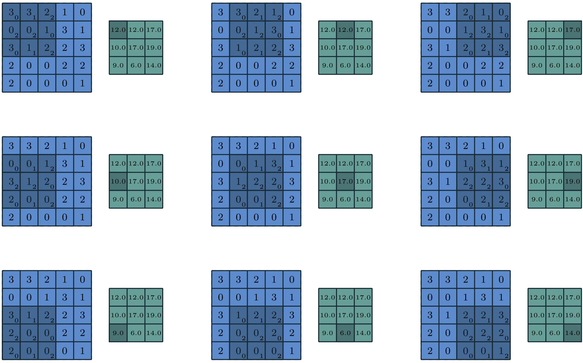The table above shows two examples of 2D convolution without flipping the kernel. The output is restricted to positions where the kernel fits entirely inside the image; this type of operation is sometimes called a “valid” convolution.