This note provides a structured overview of the main neural network architectures and related modeling paradigms used in deep learning. The purpose is not to derive the underlying mathematics in detail, but to clarify what each family is designed for, what its core inductive bias is, and why it became important in practice.
Abstract
The term architecture is used here in a broad sense. Some entries refer to precise neural designs, such as CNNs or Transformers, while others refer to broader learning frameworks, such as Deep Reinforcement Learning or Physics-Informed Neural Networks.
Note
These categories should not be interpreted as mutually exclusive. Modern systems are often hybrid: a model may combine convolutional layers with attention, use a Transformer inside a reinforcement learning pipeline, or integrate graph neural networks into a larger multimodal architecture.
Warning
This overview is broader than the set of topics developed in detail on this site. Some families are included for orientation only. In particular, Autoencoders, GANs, Deep Reinforcement Learning, and Physics-Informed Neural Networks (PINNs) will not be covered extensively in later sections.
1. Autoencoders
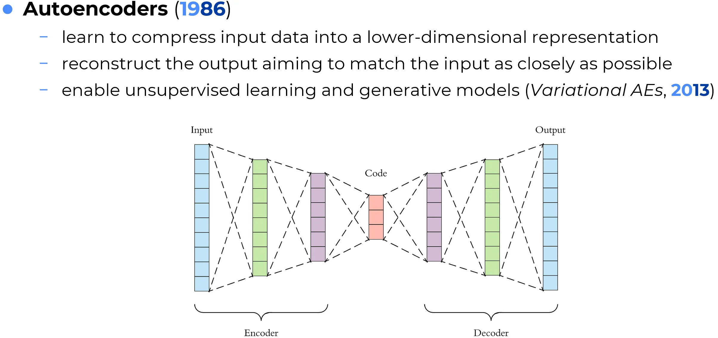
Autoencoders are neural networks trained to reproduce their input at the output after passing it through an internal compressed representation. Their standard structure consists of two parts: an encoder, which maps the input into a latent code, and a decoder, which reconstructs the original data from that code. The learning objective is usually based on reconstruction error, such as mean squared error for continuous data or binary cross-entropy for binary-valued inputs.
The central idea is that if a model is forced to reconstruct the input through a bottleneck, it must learn a compact and informative internal representation rather than simply memorizing the raw data. In this sense, autoencoders are one of the classical tools of representation learning.
Autoencoders are important because they provide a way to learn useful latent features without requiring manually labeled targets. They have historically been used for dimensionality reduction, denoising, anomaly detection, feature extraction, and learned data compression. In more advanced forms, they also became foundational to generative modeling, especially through Variational Autoencoders (VAEs), which impose a probabilistic structure on the latent space.
Historical Curiosity: Learned Compression Surpassed Top Hand-Engineered Codecs
A major milestone in learned image compression was reached in 2018, when autoencoder-based encoder-decoder systems became competitive with, and in some benchmark settings better than, leading hand-engineered codecs such as BPG (Better Portable Graphics).
Two particularly important papers were:
- Johannes Ballé, David Minnen, Saurabh Singh, Sung Jin Hwang, and Nick Johnston, Variational Image Compression with a Scale Hyperprior (ICLR 2018)
- David Minnen, Johannes Ballé, and George Toderici, Joint Autoregressive and Hierarchical Priors for Learned Image Compression (NeurIPS 2018)
These models were not plain autoencoders in the simplest sense. They combined an autoencoder-style latent representation with quantization, entropy modeling, and arithmetic coding. The encoder learned how to map an image into a compact latent code, while the decoder reconstructed the image from that compressed representation. The entire system was trained end-to-end to optimize the rate-distortion tradeoff, that is, the balance between file size and reconstruction quality.
The significance of this result is conceptual as much as practical. Traditional codecs such as JPEG, JPEG2000, WebP, and BPG were designed through hand-engineered signal-processing principles. Learned compression showed that the transform itself could be discovered from data. In particular, the 2018 work of Minnen, Ballé, and Toderici reported a learned method that outperformed BPG on both PSNR and MS-SSIM under the evaluation setting used in the paper.
This claim should still be read carefully. A basic autoencoder does not universally beat every classical codec: performance depends on the dataset, bitrate regime, distortion metric, and computational budget. The accurate, narrower statement is that learned latent compression became strong enough to surpass top human-engineered codecs on important benchmarks.
Sources. Both papers (Ballé et al., 2018; Minnen, Ballé, Toderici, 2018) are catalogued under Learned Image Compression in the literature section of this site.
Important
An autoencoder is more than a compression tool: its real value lies in learning a latent representation that preserves the information necessary to reconstruct the data while filtering out irrelevant variation.
A linear autoencoder rediscovers PCA
Strip the nonlinearities from an autoencoder, keep a single bottleneck layer of width , and train it under mean-squared reconstruction error. The optimum is not an arbitrary compression: the encoder spans exactly the subspace of the top principal components of the data (Baldi and Hornik, 1989), and the reconstruction is the orthogonal projection onto that subspace, which is what PCA computes. Nonlinear autoencoders earn their keep by bending this flat subspace into a curved low-dimensional manifold, but the linear case fixes the intuition: the bottleneck is a learned, and in general nonlinear, generalization of principal component analysis.
2. Convolutional Neural Networks
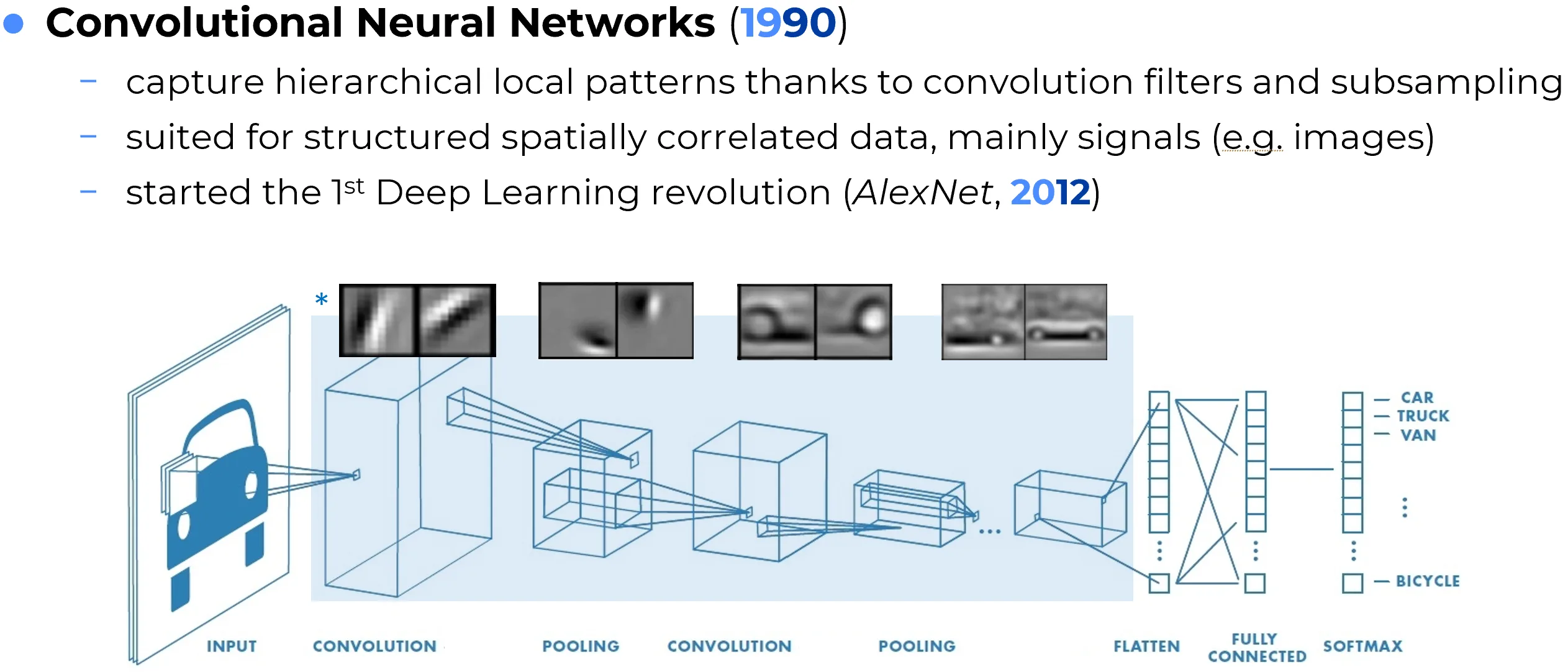
Convolutional Neural Networks (CNNs) are neural architectures specifically designed for data with strong local spatial structure, especially images. Their defining operation is the convolution, in which a small learnable filter is applied across the input to detect local patterns such as edges, textures, corners, or repeated motifs.
The major inductive bias of CNNs is that the same visual pattern may appear in different spatial positions. Instead of learning a separate weight for every pixel and every location, convolutional layers reuse the same filters across the image. This parameter sharing makes CNNs far more efficient than fully connected networks for visual tasks and allows them to exploit translation-related regularities in natural images.
As information flows through the network, early layers tend to capture simple local structures, while deeper layers combine them into more abstract concepts such as shapes, object parts, and semantic categories. Pooling operations or strided convolutions are often used to progressively reduce spatial resolution while increasing representational abstraction.
CNNs dominated computer vision for more than a decade and were central to the rise of deep learning after the success of AlexNet (2012). They remain important in image classification, object detection, segmentation, medical imaging, audio spectrogram analysis, and many scientific applications involving grid-like data.
Tip
A useful way to think about CNNs is as feature extractors for structured spatial signals, with image classification being only the most familiar use.
Convolution and attention are two ends of one spectrum
A convolution mixes each location with its neighbours using a fixed kernel, the same weights everywhere, chosen independently of the pixel values. Self-attention mixes each position with the others using weights computed from the content itself, with no locality restriction. Placed side by side, a convolution is attention with a hard-coded, local, input-independent weighting, and attention is a convolution whose kernel is generated on the fly from the data and allowed to span the whole input. This is why a Vision Transformer can in principle subsume a CNN: it can represent the convolutional weighting as one special case, but it gives up the strong locality bias and therefore needs far more data to match a CNN’s efficiency on images.
3. Recurrent Neural Networks
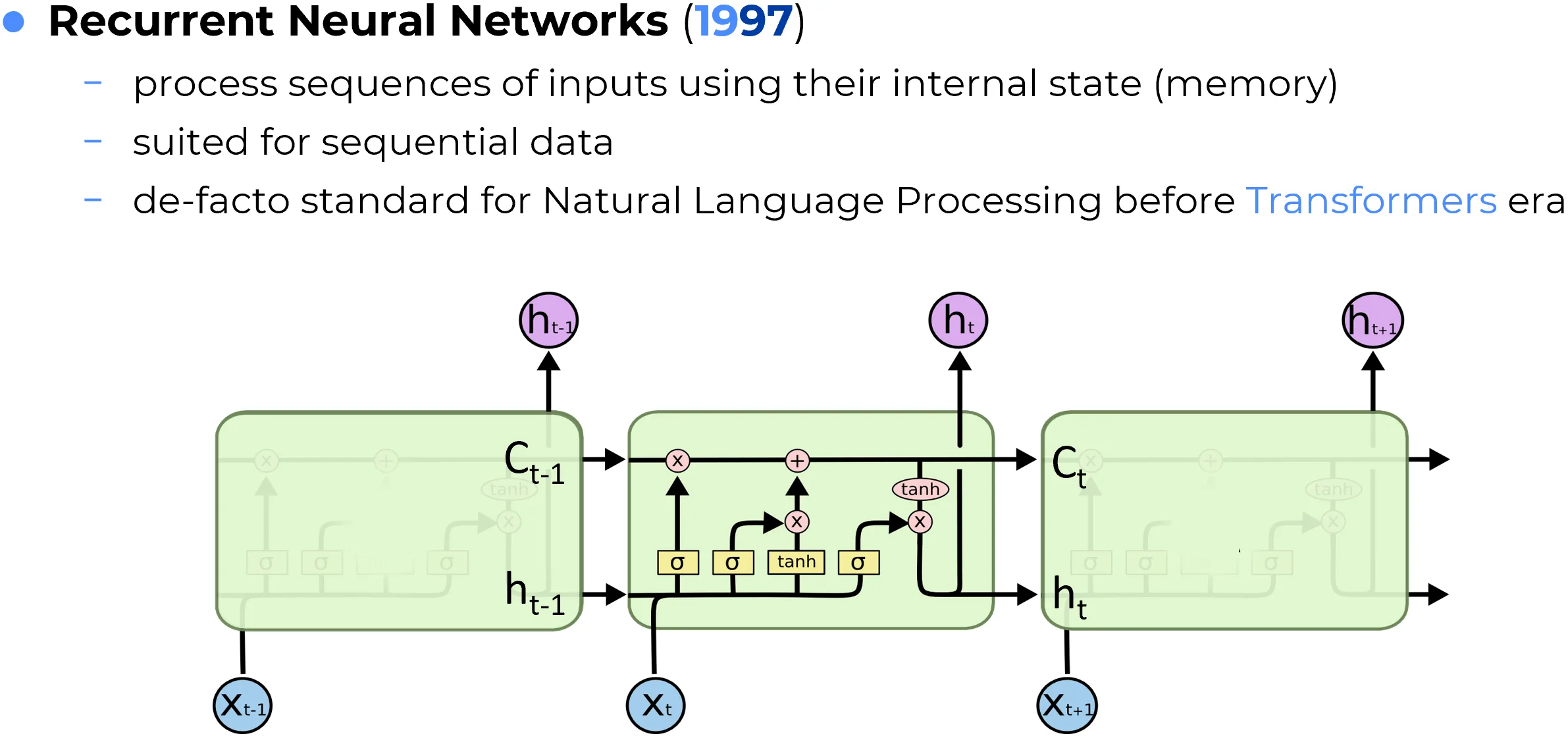
Recurrent Neural Networks (RNNs) are designed for sequential data, where the order of observations matters. Instead of processing the entire input at once, an RNN reads the sequence step by step and maintains a hidden state that acts as a running summary of the past. This makes recurrent models naturally suited for language, speech, time series, and other temporally ordered signals.
The key intuition is that the interpretation of the current element often depends on what came before. In a sentence, for example, the meaning of a word may depend on its context; in a time series, the current value may depend on previous states of the system. RNNs address this by using the same recurrent transformation at every time step, thereby creating a form of parameter sharing through time.
Standard or “vanilla” RNNs were conceptually elegant but difficult to train on long sequences because of the vanishing and exploding gradient problem. This limitation motivated more robust recurrent designs such as Long Short-Term Memory (LSTM) networks and Gated Recurrent Units (GRUs), which introduced gating mechanisms that regulate what information should be stored, updated, or forgotten.
Before the widespread adoption of Transformers, recurrent networks were the dominant architecture for natural language processing, speech recognition, and many sequential prediction tasks. Even today, they remain relevant in settings where strict temporal causality, low-latency streaming, or compact recurrent state is desirable.
Note
RNNs introduced one of the central ideas in deep learning for sequences: the same model can be reused across an arbitrary number of time steps while maintaining a learned memory of the past.
The fixed-state bottleneck, now a selling point again
An RNN compresses the entire history into a hidden state of fixed size. Each new token overwrites part of that finite memory, which is the deep reason long-range dependencies are hard: the past is summarized lossily before the model knows what it will need. Attention made the opposite choice, keeping every past token available at a cost of compute and memory. The trade is clean: bounded state with linear-time inference against unbounded memory with quadratic cost. This is why state-space models such as Mamba revived the recurrent design for very long sequences, where attention’s quadratic cost becomes the binding constraint.
4. Transformers
Transformers are neural architectures based primarily on attention mechanisms, rather than recurrence or convolution, for modeling dependencies within sequences. Their central innovation is the use of self-attention, which allows each token in a sequence to directly interact with every other relevant token when building its contextual representation.
This design has two major consequences. First, it allows long-range dependencies to be modeled far more effectively than in standard recurrent systems, where information must propagate step by step through time. Second, it makes training highly parallelizable, since all sequence positions can be processed simultaneously rather than sequentially. This compatibility with modern GPU and TPU hardware is one of the key reasons Transformers scaled so successfully.
In the canonical architecture introduced in Attention Is All You Need (2017), the model combines self-attention, feed-forward layers, positional encodings, residual connections, and normalization. In encoder-decoder settings, such as machine translation, cross-attention is also used to let the decoder attend to the encoded source sequence.
Transformers became the dominant architecture in natural language processing and later expanded to vision, audio, biology, robotics, and multimodal modeling. Large Language Models (LLMs), vision transformers, multimodal assistants, and many foundation models are all built on Transformer-based principles.
Important
The Transformer was more than a better sequence model: it changed the scaling regime of deep learning by aligning model design with large datasets, distributed training, and hardware-efficient parallel computation.
A Transformer is a graph neural network on a fully connected graph
Self-attention treats the input as a set of tokens with an edge between every pair and updates each token by aggregating messages from all the others, weighted by attention scores. That is precisely the message-passing computation of a graph neural network (Section 7), specialized to the complete graph with content-based edge weights; the positional encoding restores the order that the set view discards. Read together, CNNs (grid graph, fixed weights), GNNs (arbitrary graph, learned weights) and Transformers (complete graph, attention weights) are three instances of the same neighbourhood-aggregation template, differing only in which graph they run on and how they weight the edges.
5. GANs
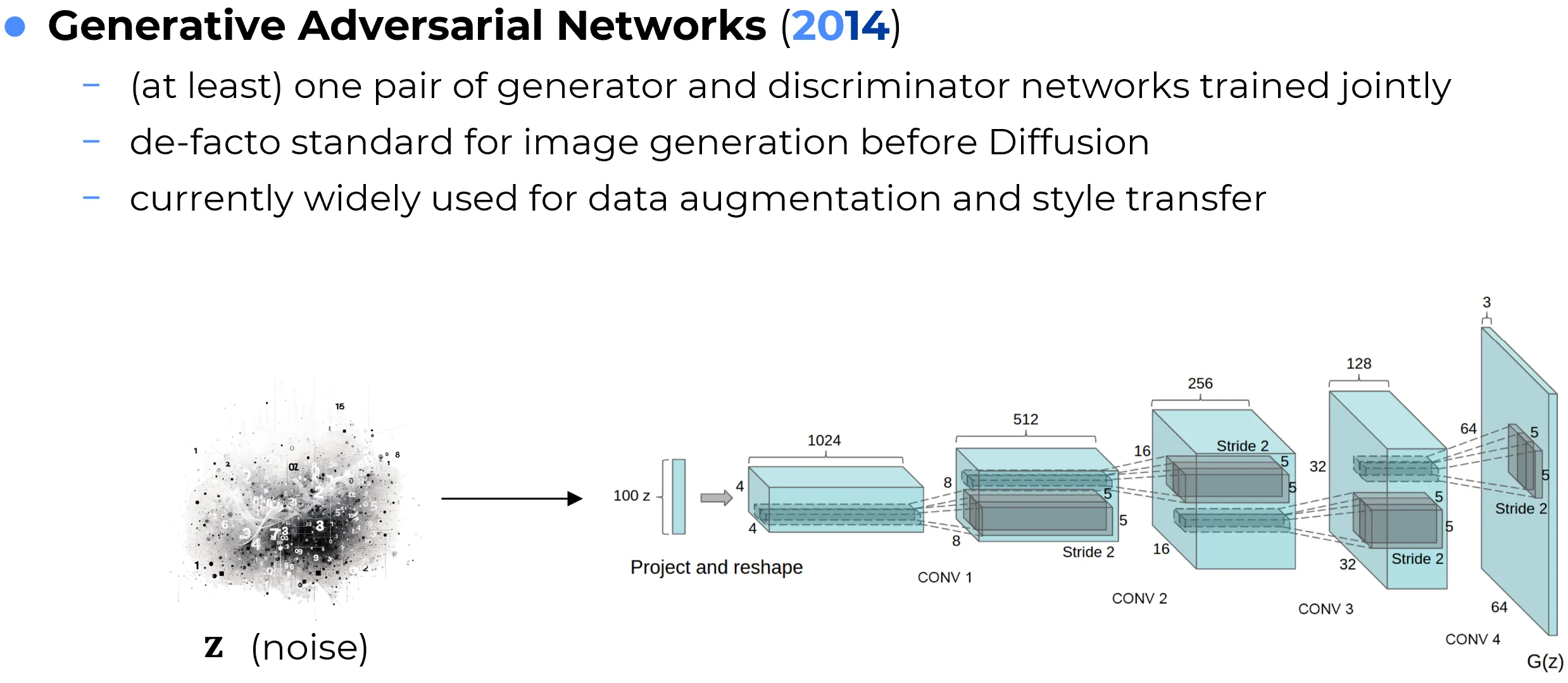
Generative Adversarial Networks (GANs) are generative models based on a competitive game between two neural networks: a generator, which tries to produce realistic synthetic samples, and a discriminator, which tries to distinguish real samples from generated ones. The generator improves by learning to fool the discriminator, while the discriminator improves by learning to detect the generator’s mistakes.
This adversarial setup makes GANs very different from likelihood-based generative models. Rather than explicitly maximizing the probability of the data, GANs learn to produce outputs that are difficult to distinguish from real examples. When training succeeds, the generator can produce highly sharp and realistic samples, especially in image domains.
GANs became influential in image synthesis, image-to-image translation, super-resolution, style transfer, face generation, data augmentation, and domain adaptation. Architectures such as DCGAN, CycleGAN, StyleGAN, and related variants demonstrated that generative models could produce visually compelling outputs far beyond what earlier methods achieved.
At the same time, GANs are notoriously difficult to train. Practical issues such as instability, mode collapse, sensitivity to hyperparameters, and fragile equilibrium between generator and discriminator made them powerful but often hard to control. For this reason, diffusion models later displaced GANs in many mainstream generative tasks, especially where sample diversity and training robustness are critical.
Warning
GANs are best understood as a training framework for generation, not as a single fixed neural architecture. The defining idea is adversarial learning.
The discriminator is a learned loss function
The reason GAN samples look sharp while autoencoder and VAE reconstructions look blurry comes down to the loss. A pixel-wise mean-squared error rewards predicting the average of all plausible outputs, and the average of many sharp images is a blurry one. The discriminator replaces that fixed averaging loss with an adaptive one: it learns to penalize whatever currently separates fakes from real data, so blur, an easy giveaway, is punished directly. A GAN is in this sense a generator trained against a loss that trains itself, which is also the root of its instability: the objective keeps moving as the discriminator adapts.
6. Diffusion Models
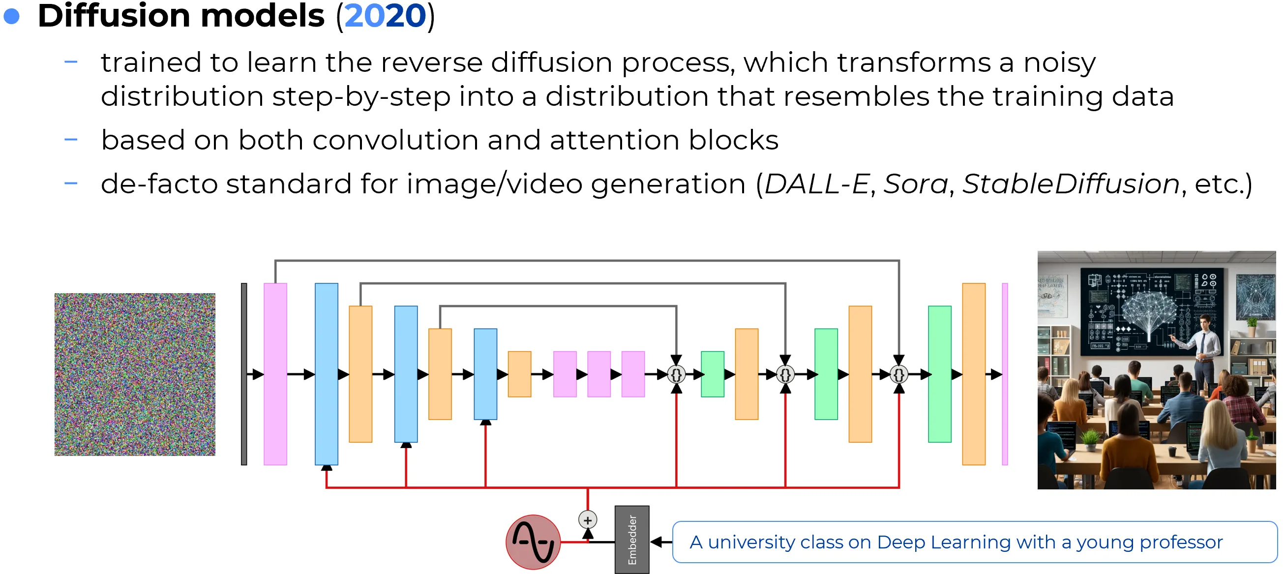
Diffusion models are generative models that learn to reverse a gradual corruption process. During training, data is progressively perturbed by noise until it becomes nearly random. The model then learns how to predict and remove that noise step by step. At generation time, the process starts from random noise and iteratively denoises it into a coherent sample.
The conceptual advantage of diffusion models is that generation is decomposed into many small and stable refinement steps rather than a single direct mapping from latent noise to output. This often leads to highly realistic samples, strong mode coverage, and more stable training behavior than GANs.
Diffusion models became especially prominent in image generation, where they power many state-of-the-art systems for text-to-image synthesis, image editing, inpainting, and controllable generation. They have also been extended to audio, video, molecules, and scientific domains.
Although they can be computationally expensive due to iterative sampling, many improvements have been developed to accelerate inference and make them practical at scale. In the modern generative landscape, diffusion models are one of the central paradigms alongside autoregressive Transformers.
Important
Diffusion models illustrate a broader principle in generative modeling: high-quality synthesis can emerge from repeated denoising and gradual refinement rather than direct one-shot generation.
Diffusion is a very deep autoencoder whose encoder does no learning
The forward noising process is an encoder that maps data to noise, except it carries no parameters: it is a fixed Gaussian corruption. The reverse process is a decoder trained to undo one small step at a time. A diffusion model is therefore close to a hierarchical VAE (Section 1) with hundreds of latent levels and a frozen, hand-designed encoder. Freezing the encoder removes the hardest part of training a deep latent-variable model, learning the encoder and decoder jointly, and replaces it with many small, well-conditioned denoising regressions.
The generative trilemma
Three properties are wanted from any generative model: high sample quality, broad mode coverage, and fast sampling. In practice only two are obtained at once (Xiao et al., 2021). GANs reach quality and speed but can collapse to a few modes; diffusion reaches quality and coverage but samples slowly through many steps; VAEs and normalizing flows sample fast with good coverage but blurrier quality. Much of modern generative research is an attempt to buy back the missing corner, for instance by distilling a slow diffusion model into a few-step sampler.
7. Graph Neural Networks
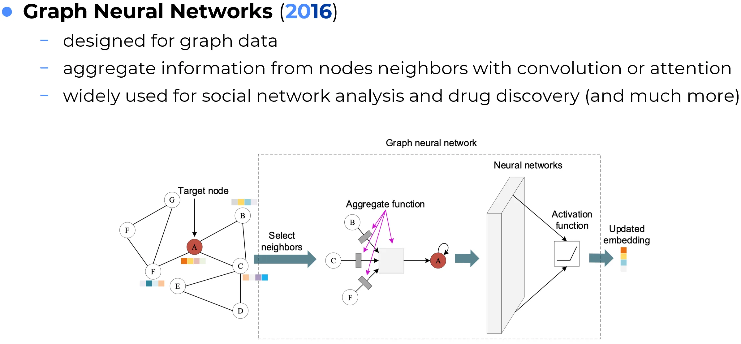
Graph Neural Networks (GNNs) are neural architectures designed for graph-structured data, where information is represented as nodes connected by edges. Unlike images or sequences, graphs do not have a regular grid structure, so standard convolutions or recurrent schemes are not directly appropriate.
The core idea behind most GNNs is message passing. Each node updates its representation by collecting, transforming, and aggregating information from its neighboring nodes. By stacking multiple layers, a node can incorporate information from progressively larger neighborhoods, allowing the model to reason over relational structure.
This makes GNNs especially useful for domains in which the relationships between entities are more important than their isolated features. Typical applications include molecular property prediction, recommender systems, knowledge graphs, fraud detection, traffic networks, and social graph analysis.
Different GNN variants implement message passing in different ways. Some use simple normalized aggregation, as in Graph Convolutional Networks (GCNs), while others use learned attention weights, as in Graph Attention Networks (GATs). The broader goal is always to exploit relational inductive bias: the idea that connected entities influence one another.
Note
GNNs extend deep learning beyond Euclidean domains. Their importance lies in making neural computation compatible with structured relational data.
Why GNNs stay shallow while CNNs go deep
Stacking convolutional layers reliably helps; stacking message-passing layers usually hurts beyond a few. Each GNN layer averages a node with its neighbours, and repeated averaging is a diffusion that pulls all embeddings toward the same vector, so after a handful of layers connected nodes become indistinguishable. This failure, called oversmoothing, caps most GNNs at two to four layers, in sharp contrast to the hundred-layer CNNs that residual connections made trainable. A related obstacle, oversquashing, is that an exponentially growing neighbourhood is forced through a fixed-size node vector, so distant information arrives compressed to the point of being unusable.
8. Deep Reinforcement Learning
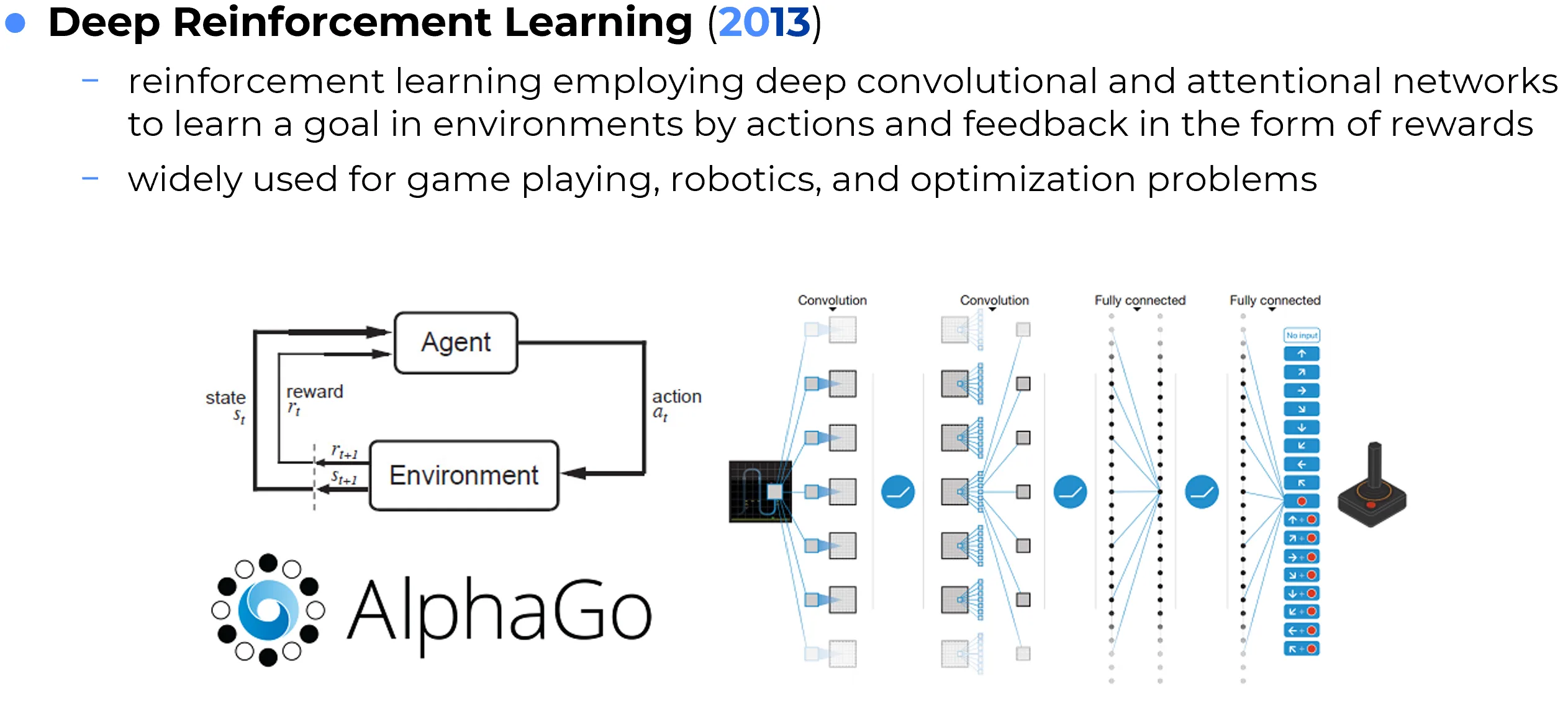
Deep Reinforcement Learning (Deep RL) combines neural networks with reinforcement learning, a framework in which an agent learns through trial and error by interacting with an environment and receiving rewards or penalties. Instead of being trained only on static labeled examples, the agent must discover which actions lead to desirable long-term outcomes.
Neural networks play different roles in this setting. They may approximate a policy that maps states to actions, a value function that estimates expected future reward, or a more structured internal model of the environment. This combination allows reinforcement learning to scale to high-dimensional state spaces such as images, sensor streams, or game observations.
Deep RL became widely known through systems that learned to play Atari games, master Go, control robots, or optimize sequential decision problems. Its importance lies in extending deep learning from pattern recognition to sequential decision-making under uncertainty.
However, Deep RL is not a single architecture. It is better understood as a learning paradigm in which many architectures can be used depending on the problem. CNNs are common for visual input, recurrent models are useful under partial observability, and Transformers are increasingly used in modern policy learning and world modeling.
Important
Deep RL is defined by the learning setup, not by a unique network structure. Its central question is not “what label should be predicted?” but “what action should be taken to maximize long-term reward?”
The deadly triad
Three ingredients are each safe in isolation yet tend to diverge together: function approximation (a neural network for the value), bootstrapping (updating an estimate from other estimates, as in temporal-difference learning) and off-policy training (learning about one policy from data generated by another). Sutton and Barto call this combination the deadly triad, and Deep RL lives inside it, which is much of why it is so much less stable than supervised deep learning. Several of its signature devices, target networks, experience replay and conservative clipping, exist mainly to tame the triad rather than to add capacity.
9. Physics-Informed Neural Networks
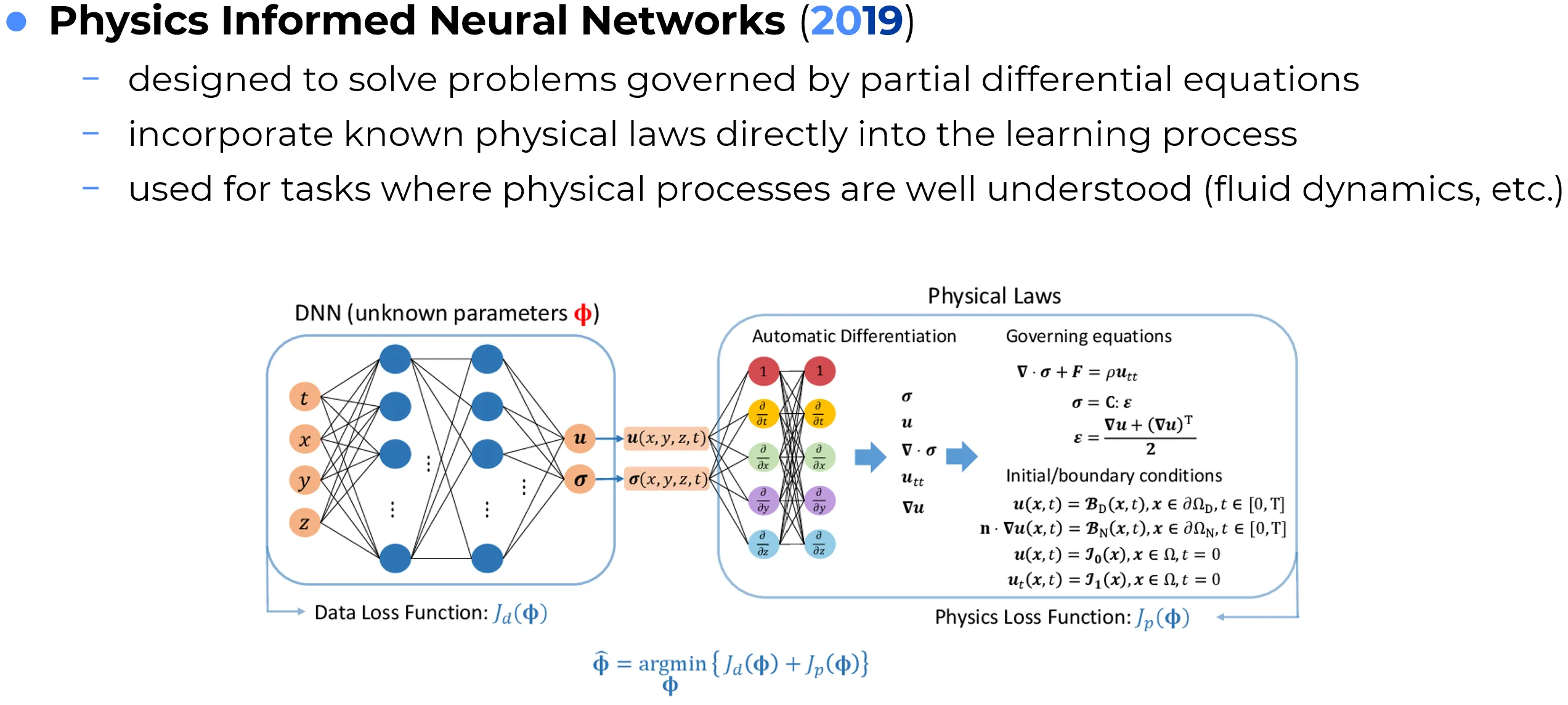
Physics-Informed Neural Networks (PINNs) are neural models trained not only on observational data, but also under explicit physical constraints. These constraints are usually incorporated into the loss function by penalizing violations of governing equations, such as ordinary or partial differential equations, as well as boundary and initial conditions.
The motivation is clear: in many scientific and engineering problems, pure data-driven learning is inefficient or unreliable because the available data is limited, expensive, noisy, or incomplete. If relevant physical laws are already known, it is advantageous to force the model to respect them during training.
PINNs are used in scientific computing, fluid dynamics, inverse problems, system identification, surrogate modeling, and other tasks where one wants a neural approximation that remains consistent with established physical principles. In this sense, they represent an important bridge between machine learning and computational physics.
Like Deep RL, PINNs are not one fixed architectural family in the narrow sense. The defining feature is not a specific layer type, but the way domain knowledge is integrated into optimization. Their significance lies in showing that neural networks do not have to learn only from examples; they can also be shaped by theoretical structure.
Tip
A useful way to understand PINNs is as constrained function approximators: they learn from data, but they are simultaneously pushed to remain compatible with known equations.
Two limits worth knowing, and the operator alternative
First, ordinary networks have a spectral bias: they fit low-frequency structure long before high-frequency detail, so PINNs converge slowly on solutions with sharp gradients or stiff, multi-scale behaviour, exactly the regimes where classical solvers already excel. Second, a trained PINN solves a single boundary-value problem; changing an initial condition or a coefficient requires retraining. This motivated neural operators (DeepONet, the Fourier Neural Operator), which learn the solution map of an entire family of PDEs at once, trading the per-instance physics constraint for a learned mapping between function spaces.
10. Summary
These architecture families can be organized according to the type of structure or problem they are designed to address:
- Autoencoders learn compact latent representations through reconstruction.
- CNNs exploit local spatial structure in grid-like data such as images.
- RNNs model temporal and sequential dependencies through recurrent state updates.
- Transformers use attention to build context-rich representations at scale.
- GANs and Diffusion Models are central paradigms for generative modeling.
- GNNs operate on relational and graph-structured data through message passing.
- Deep RL addresses decision-making through reward-driven interaction.
- PINNs integrate scientific constraints directly into the learning process.
Abstract
The broader lesson is that neural network design is guided by inductive bias. Different architectures become useful because they encode different assumptions about the structure of data, the nature of the task, and the kind of computation required to solve it.
One principle behind the catalogue: symmetry dictates architecture
Most of these families answer a single question: what changes to the input should leave the answer essentially unchanged? Translating an image does not change which object it shows, so CNNs share weights across space. Shifting a sequence in time reuses the same rule, so RNNs share weights across time. Permuting the nodes of a graph or the tokens of a set should permute the output the same way, so GNNs and Transformers are built to be permutation-equivariant. In each case the symmetry of the data decides which weights are tied together, and weight sharing is the mechanism that enforces it. This is the organizing idea of geometric deep learning (Bronstein et al., 2021): an architecture is a hypothesis about the symmetries of its domain, and its inductive bias is a good one precisely when those symmetries match the data.