bp-mlp-3

An equation for the error in the output layer

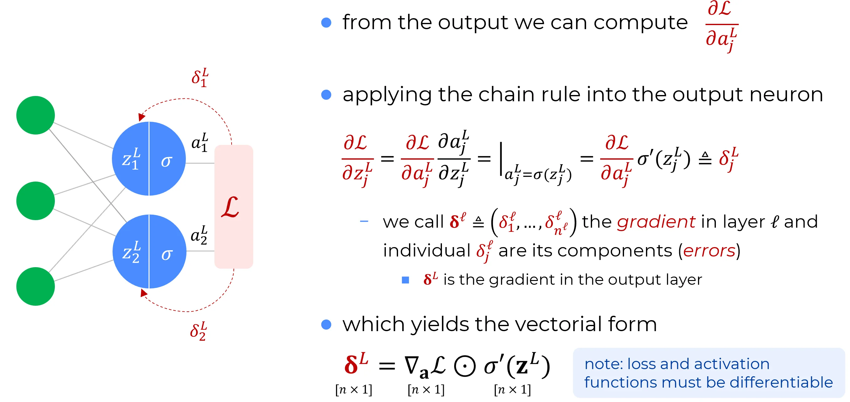
The components of ${\delta }^L$ are given by

$$\boxed{{\delta }_j^L=\frac{\partial \mathcal{L}}{\partial a_j^L}{\sigma }^{\prime }(z_j^L)}\text{\hspace{1em}(BP1)}$$

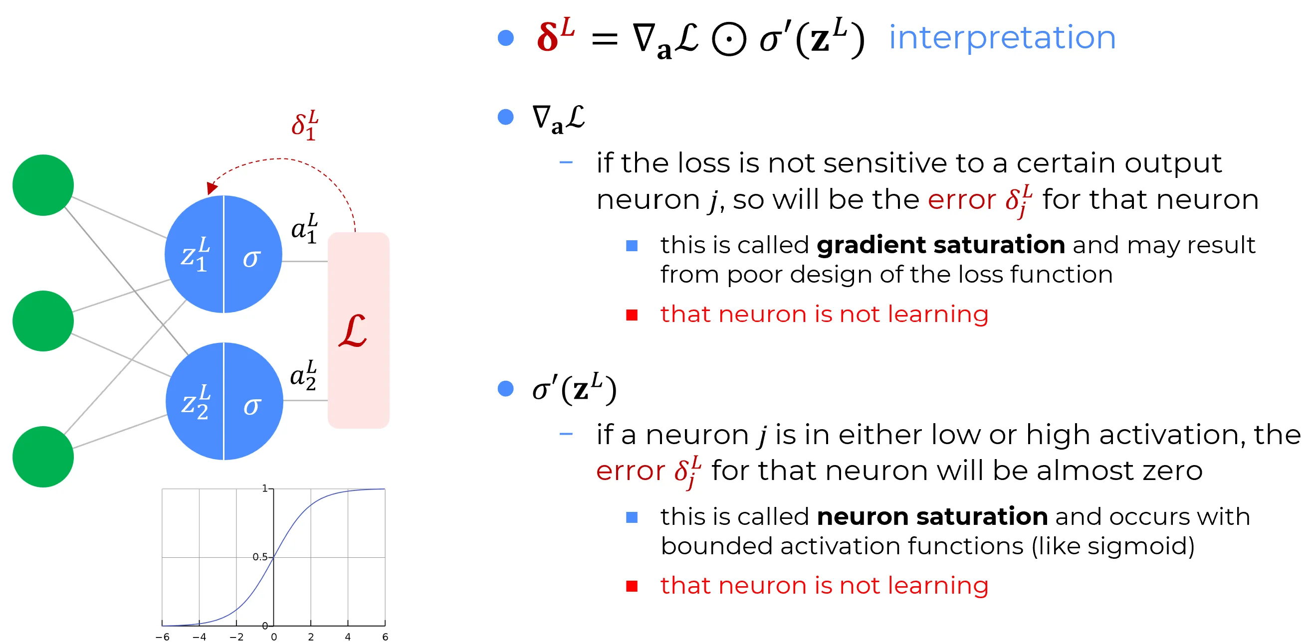
This is a very natural expression:

• the first term on the right, $\partial \mathcal{L}/\partial a_j^L$, just measures how fast the cost is changing as a function of the $j-th$ output activation. If, for example, $\mathcal{L}$ doesn’t depend much on a particular output neuron, $j$, then ${\delta }_j^L$ will be small, which is what we’d expect.

• the second term on the right, ${\sigma }^{\prime }(z_j^L)$, measures how fast the activation function $\sigma$ is changing at $z_j^L$

Notice that everything in Eq. $\text{ref}eq:BP1$ equation is easily computed. In particular, we compute $z_j^L$ while computing the behavior of the network, and it’s only a small additional overhead to compute ${\sigma }^{\prime }(z_j^L)$. The exact form of $\partial \mathcal{L}/\partial a_j^L$ will, of course, depend on the form of the cost function. However, provided the cost function is known there should be little trouble computing $\partial \mathcal{L}/\partial a_j^L$. For example, if we’re using the quadratic cost function then $\mathcal{L}=\frac{1}{2}{\sum }_j(y_j-a_j^L{)}^2$, and so $\partial \mathcal{L}/\partial a_j^L=(a_j^L-y_j)$, which obviously is easily computable.

Equation~(\ref{eq:BP1}) is a component wise expression for ${\delta }^L$. It’s a perfectly good expression, but not the matrix-based form we want for backpropagation. However, it’s easy to rewrite the equation in a matrix-based form, as

$${\delta }^L={\nabla }_a\mathcal{L}\odot {\sigma }^{\prime }(z^L)\text{\hspace{1em}(BP1a)}$$

Here, ${\nabla }_a\mathcal{L}$ is defined to be a vector whose components are the partial derivatives $\partial \mathcal{L}/\partial a_j^L$. You can think of ${\nabla }_a\mathcal{L}$ as expressing the rate of change of $\mathcal{L}$ with respect to the output activations. It’s easy to see that Equations (\ref{eq:BP1a}) and (\ref{eq:BP1}) are equivalent, and for that reason from now on we’ll use (\ref{eq:BP1}) interchangeably to refer to both equations. As an example, in the case of the quadratic cost we have ${\nabla }_a\mathcal{L}=(a^L-y)$, and so the fully matrix-based form of (\ref{eq:BP1}) becomes

$${\delta }^L=(a^L-y)\odot {\sigma }^{\prime }(z^L)$$

As you can see, everything in this expression has a nice vector form, and is easily computed using a library such as Numpy.

---

Interpretation