Stochastic GD (SGD)

Several challenges arise in the practical application of the gradient descent rule, many of which will be examined in detail later. At this stage, however, it is useful to highlight one key difficulty.

Consider the quadratic loss introduced earlier. This loss has the form

$$\mathcal{L}=\frac{1}{n}\sum _x{\mathcal{L}}_x,$$

where the individual contribution for a training example $x$ is defined as if $\mathcal{L}$ is the MSE

$${\mathcal{L}}_x\equiv \frac{1}{2}\Vert y(x)-a{\Vert }^2.$$

In practice, computing the full gradient $\nabla \mathcal{L}$ requires first evaluating the gradients $\nabla {\mathcal{L}}_x$ for each individual training input $x$, and then averaging them:

$$\nabla \mathcal{L}=\frac{1}{n}\sum _x\nabla {\mathcal{L}}_x.$$

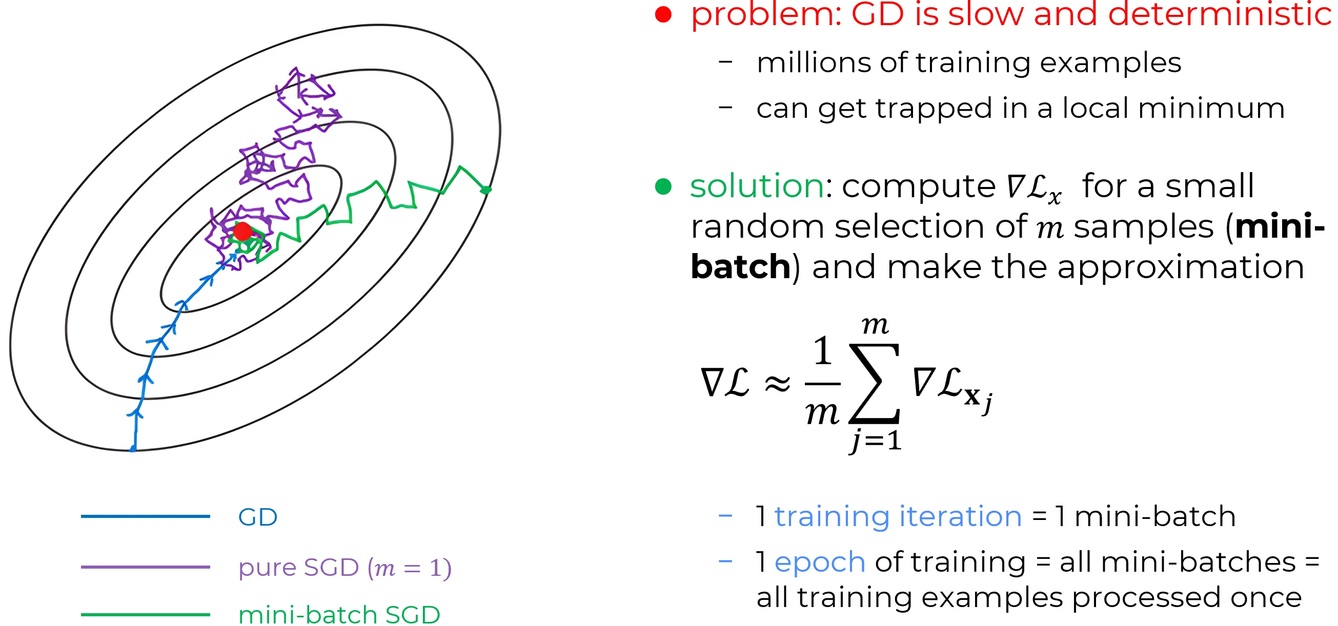
When the training set is very large, this computation becomes prohibitively time-consuming, and as a result the learning process proceeds very slowly.

A widely used strategy for addressing this computational bottleneck is stochastic gradient descent (SGD).
The central idea is to approximate the full gradient $\nabla \mathcal{L}$ by computing it on a small, randomly selected subset of the training data, rather than over the entire dataset.

Concretely, suppose a subset of $m$ training examples is sampled at random, denoted $X_1,X_2,\dots ,X_m$. This subset is referred to as a mini-batch.
For each example $X_j$, the corresponding gradient $\nabla {\mathcal{L}}_{X_j}$ is computed.
If $m$ is sufficiently large, the average of these gradients provides a good approximation to the true gradient:

$$\frac{1}{m}\sum _{j=1}^m\nabla {\mathcal{L}}_{X_j}\approx \frac{1}{n}\sum _x\nabla {\mathcal{L}}_x=\nabla \mathcal{L}.$$

Equivalently,

$$\nabla \mathcal{L}\approx \frac{1}{m}\sum _{j=1}^m\nabla {\mathcal{L}}_{X_j}.$$

Thus, by averaging over a randomly chosen mini-batch, an efficient and reasonably accurate estimate of the full gradient can be obtained, significantly accelerating the learning process.

To make the connection with neural networks explicit, let $w_k$ and $b_l$ denote the weights and biases, respectively.
Under stochastic gradient descent, training proceeds by selecting a randomly chosen mini-batch of inputs and updating the parameters according to

$$w_k^{\prime }=w_k-\eta \frac{1}{m}\sum _{j=1}^m\frac{\partial {\mathcal{L}}_{X_j}}{\partial w_k},$$ $$b_l⟶b_l^{\prime }=b_l-\eta \frac{1}{m}\sum _{j=1}^m\frac{\partial {\mathcal{L}}_{X_j}}{\partial b_l},$$

where the sums extend over all training examples $X_j$ in the current mini-batch.
Once this mini-batch has been processed, a new mini-batch is drawn at random, and the process is repeated.
After all training examples have been used once, an epoch of training is said to be complete, after which the cycle begins again.

Convention on Scaling

Conventions vary regarding the scaling of the loss function and the mini-batch updates.

• In the earlier quadratic loss definition, the cost function was scaled by a factor of $\frac{1}{n}$. In other contexts, the cost is written as a direct sum over training examples, omitting this factor. This convention is particularly useful when the total number of training examples is not fixed in advance—for instance, when new data is generated in real time.
• Similarly, the update rules above include the factor $\frac{1}{m}$ to average over the mini-batch. Some formulations omit this term, which is conceptually equivalent to rescaling the learning rate $\eta$.

While these differences are not mathematically fundamental, they must be carefully noted when comparing results across different works or implementations.