Vanilla RNNs limitations

The basics section ended with a diagnosis: a vanilla RNN trained by Backpropagation Through Time cannot reliably learn long-range dependencies, because its recurrent Jacobian product either vanishes or explodes geometrically with the temporal gap (the analysis is in BPTT Problems). Gradient Clipping tames the exploding side, and BPTT Variants bound the cost of the unrolled computation, but neither closes the gap between the truncation horizon $K$ and the actual timescale of the data. The problem is architectural.

This section develops the architectural fix.

The story arc

1. Vanilla RNNs limitations turns the gradient analysis into a precise architectural diagnosis: the vanilla cell cannot preserve information because it has no stable way to leave a value alone. It then sketches the fix, an additively-updated memory gated by a learned forget gate, which is the seed of the LSTM.
2. LSTM Layer (the subfolder) builds the cell one gate at a time: the cell state as a temporal skip connection, then the forget, input and output gates, then the complete forward pass and mini-batch form in Putting all together.
3. Gradient in LSTM returns to the gradient analysis with the full cell in hand, and shows mathematically why the cell-state line carries gradient across arbitrary horizons.

Across the three parts a single mathematical fact does almost all the work: the recurrent Jacobian along the cell state is the diagonal forget-gate matrix $\mathrm{diag}({\mathbf{f}}_t)$, not a product of dense matrices and saturating slopes. The notes spell out the consequences of that one fact from every angle the architecture exposes.

What to expect

The treatment is mathematical but not formalistic. Every gate is introduced together with the role it plays in the cell state update, the activation chosen for it, and the per-coordinate interpretation it admits. Each note carries a dimensions table for the actors that appear in it, and collapsible derivations for the steps a reader might want to verify line by line. The complete parameter count, initialization conventions, and the fused-weight implementation used by modern frameworks are collected in Putting all together.

The architectural pattern that emerges, an identity highway carrying state across the recurrence with learned modules perturbing but not overwriting it, predates by nearly two decades the residual connections that later enabled very deep feedforward networks. Reading the LSTM as the temporal special case of that pattern is the cleanest way to see why it works and why the same idea recurs throughout modern deep learning.

---

A vanilla RNN cannot reliably learn long-range dependencies. As established in BPTT Problems, the gradient that connects a distant past to the present is a product of recurrent Jacobians whose norm behaves like $({\gamma }_h{\sigma }_{\max }({\mathbf{W}}_{hh}){)}^{t-k}$, so it vanishes or explodes geometrically with the temporal gap. The vanishing-gradient barrier was made precise by Bengio, Frasconi and Simard (1994).

Reminder of the two factors in the bound

The product ${\gamma }_h{\sigma }_{\max }({\mathbf{W}}_{hh})$ collects two independent sources of attenuation or amplification along the recurrence, derived in detail in BPTT Problems:

• ${\gamma }_h={\max }_a|{\varphi }_h^{\prime }(a)|$, the maximum slope of the activation. For $\tanh$, ${\gamma }_h=1$, attained only at $a=0$; everywhere else $|{\varphi }_h^{\prime }(a)|<1$, so the activation never amplifies and almost always attenuates.
• ${\sigma }_{\max }({\mathbf{W}}_{hh})$, the spectral norm (largest singular value) of the recurrent weight matrix. It is the largest factor by which ${\mathbf{W}}_{hh}$ can stretch any unit vector: $\Vert {\mathbf{W}}_{hh}\mathbf{v}\Vert \le {\sigma }_{\max }({\mathbf{W}}_{hh})\Vert \mathbf{v}\Vert$.

Across $t-k$ steps, submultiplicativity of the matrix norm gives the geometric bound $({\gamma }_h{\sigma }_{\max }({\mathbf{W}}_{hh}){)}^{t-k}$ on the recurrent Jacobian product. Stability of long-range gradient flow requires the base to equal exactly $1$, which is the “knife-edge” discussed below.

It is tempting to read this as a nuisance to be tuned away with a better learning rate or a luckier initialization. It is not. The limitation is architectural, and seeing exactly why is what makes the eventual fix feel inevitable rather than clever.

Why a vanilla cell cannot preserve information

Look at the update one more time:

$${\mathbf{h}}_t=\tanh ({\mathbf{W}}_{hh}{\mathbf{h}}_{t-1}+{\mathbf{W}}_{xh}{\mathbf{x}}_t+{\mathbf{b}}_h).$$

At every step the previous state ${\mathbf{h}}_{t-1}$ is multiplied by ${\mathbf{W}}_{hh}$ and squashed by $\tanh$. There is no route by which a coordinate of ${\mathbf{h}}_{t-1}$ can reach ${\mathbf{h}}_t$ unchanged. The state is not carried forward; it is overwritten at every step.

For a piece of information to survive $k$ steps, the recurrent map would have to act as the identity on that information for all $k$ steps at once: ${\mathbf{W}}_{hh}$ would need an eigenvalue of magnitude exactly $1$ along the relevant direction, and the activations would have to stay in the near-linear region of $\tanh$ the whole time. This is a knife-edge. The gradient form of the same statement is exact: stable preservation requires the effective scale

$$\gamma ={\gamma }_h{\sigma }_{\max }({\mathbf{W}}_{hh})=1$$

to hold along that direction at every step. Any deviation, however small, compounds geometrically: $\gamma <1$ quietly erases the information (vanishing), $\gamma >1$ destroys it by amplification (exploding).

Preservation is unstable, not merely hard

The vanilla cell can hold long-range information only at the exact balance $\gamma =1$, a measure-zero condition that no optimizer can maintain along every direction and every step. The two failure modes of BPTT Problems are the two sides of one fact: the vanilla recurrence has no stable way to leave a value alone.

The idea that fixes it: build the identity path

If preservation cannot be hoped for, it can be built in. Instead of overwriting the state, give the cell a separate memory ${\mathbf{c}}_t$ updated additively:

$${\mathbf{c}}_t={\mathbf{c}}_{t-1}+{\mathbf{\Delta }}_t,$$

where ${\mathbf{\Delta }}_t$ is a learned increment that depends on the current input and the previous hidden state, but not on ${\mathbf{c}}_{t-1}$. The Jacobian of this update is therefore the identity by construction,

$$\frac{\partial {\mathbf{c}}_t}{\partial {\mathbf{c}}_{t-1}}=\mathbf{I},$$

so the gradient flows backward through the memory unchanged, no matter how many steps it crosses. Where the vanilla cell multiplies by a Jacobian at every step, and the product decays or blows up, the additive memory simply adds, and the backward path becomes a clean highway. This is the constant error carousel of the original LSTM.

The contrast in one line

Vanilla recurrence: $\frac{\partial {\mathbf{h}}_t}{\partial {\mathbf{h}}_{t-1}}=\mathrm{diag}({\varphi }_h^{\prime }({\mathbf{a}}_t)){\mathbf{W}}_{hh}$, a product that generically vanishes or explodes.

Additive memory: $\frac{\partial {\mathbf{c}}_t}{\partial {\mathbf{c}}_{t-1}}=\mathbf{I}$, a product that stays exactly $\mathbf{I}$.

The fix is not a better recurrent matrix; it is removing the matrix from the carry path altogether.

A purely additive memory never forgets, so the cell state grows without bound. The remedy is a single learned forget gate ${\mathbf{f}}_t\in (0,1)$ that rescales the previous memory:

$${\mathbf{c}}_t={\mathbf{f}}_t\odot {\mathbf{c}}_{t-1}+{\mathbf{\Delta }}_t,\frac{\partial {\mathbf{c}}_t}{\partial {\mathbf{c}}_{t-1}}=\mathrm{diag}({\mathbf{f}}_t).$$

Now the recurrent Jacobian is the forget gate itself, and the network learns it. Setting ${\mathbf{f}}_t\approx 1$ keeps a memory alive across a long gap; setting ${\mathbf{f}}_t\approx 0$ discards it once it is no longer useful. The crucial shift is conceptual: preservation has become a decision the model can make, not a knife-edge it has to balance on.

This additive carry path is, structurally, a skip connection along time: information and gradient move through element-wise arithmetic, with no weight matrix on the path to attenuate them. It is the temporal analogue of the residual connections that later let feedforward networks reach hundreds of layers. The cell state as a skip connection is developed in Cell state, and the gradient analysis that shows the highway in action is in Gradient in LSTM.

What this becomes: LSTM and GRU

The additive memory plus the forget gate is the core of the Long Short-Term Memory (LSTM) cell. Two more learned gates complete it: an input gate (Input gate) that decides what to write into the memory, and an output gate (Output gate) that decides what to expose from it at each step. The mechanism is built up one gate at a time in the LSTM layer notes, starting from the cell state.

The Gated Recurrent Unit (GRU) is a later simplification that merges the cell state and the hidden state and uses two gates instead of three. It keeps the essential idea, an additively-updated memory with learned gating, at a lower parameter cost.

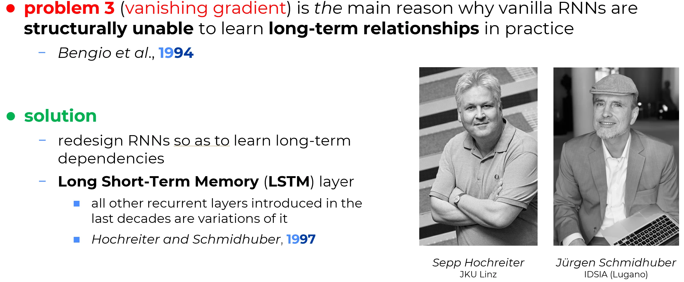
Why this mattered historically

The vanishing-gradient barrier was analysed by Bengio, Frasconi and Simard in 1994; the LSTM was proposed by Hochreiter and Schmidhuber in 1997. It became the first neural architecture to achieve large-scale commercial success. LeCun’s earlier work on handwriting recognition was commercially relevant but confined to a narrow niche, whereas LSTMs made large-vocabulary speech recognition practical. For most of the period before the modern deep-learning era, the great majority of commercially deployed neural networks were, in practice, LSTMs.