01 - Padding and Stride

Stride

Stride

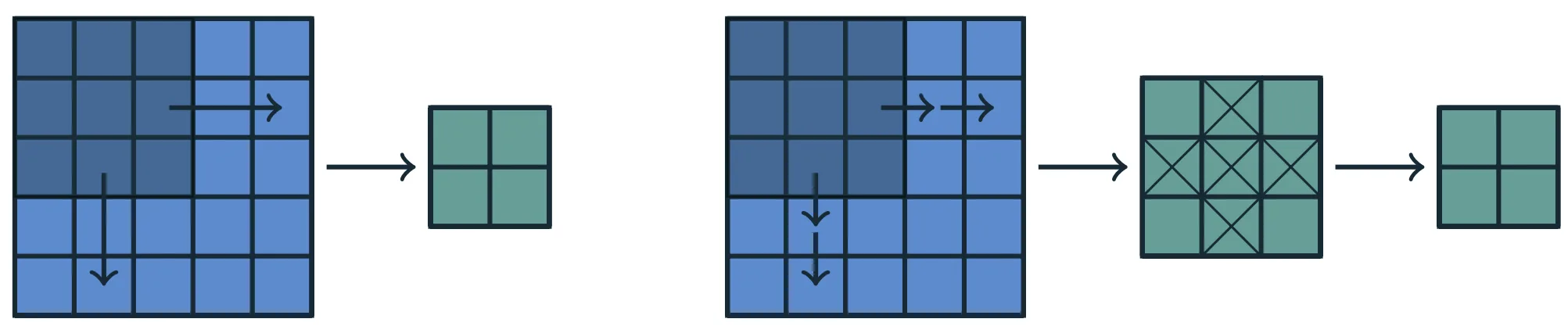
Neuroni adiacenti nel layer successivo osservano regioni diverse del layer precedente, traslate di un’unità rispetto a quella del neurone corrente:

• il neurone immediatamente a destra è sensibile a un LRF spostato di una posizione a destra;
• il neurone immediatamente sotto è sensibile a un LRF spostato di una posizione verso il basso.

Questa traslazione di una posizione prende il nome di passo (o stride) della convoluzione.
Nel caso standard, lo stride è pari a 1, cioè la finestra locale si sposta di una sola posizione alla volta lungo ogni direzione, permettendo una copertura densa e completa del dominio.

Questa struttura regolare consente al layer convoluzionale di:

• esaminare l’intero dominio 2D in modo completo e sistematico,
• conservare la relazione spaziale locale tra l’input e l’output,
• permettere la rilevazione degli stessi pattern in più posizioni.

Note

I neuroni successivi osservano regioni diverse ma parzialmente sovrapposte del layer precedente, garantendo una copertura continua del dominio bidimensionale.

---

Padding

The shift of the Local Receptive Field in all directions gives rise to a well-known problem also encountered in Image Processing.

BISOGNA AGGIUNGERE CHE PER SMEPLICITA DI TRATTAZIONE CI SI OCNCENTRA SU UN SOLO ASSE

Problem

Let’s consider a layer $\ell$ in a convolutional network under the following assumptions:

• the layer input is a $2D$ matrix,
• the kernel has a square shape $K\times K$,
• stride $S=1$ (i.e. the LRF moves one step at a time along the input)
• no extra values are added around the borders of the input.

At the boundaries of the input matrix in layer $\ell$ (which is also the output of layer $\ell -1$), the receptive field of a neuron in layer $\ell$ may extend beyond the valid region, covering positions where no neurons exist (i.e., undefined values).
This happens because, near the edges, the center of the LRF does not have enough surrounding space to include the entire $K\times K$ window.

Even away from the borders, every convolution naturally reduces the spatial extent of the representation. In this simplified setting, the output width is

$$W_{\text{out}}=W_{\text{in}}-K+1,$$

so the width shrinks by $(K-1)$ pixels at every layer (see this note).

This forces a trade-off: either use very small kernels or accept a rapid reduction in spatial extent—both scenarios that limit the expressive power of the network.

Solution: Padding

To overcome these issues, one possible solution is to apply padding, that is artificially extend the input domain, usually by surrounding it with additional values (most commonly zeros).
This ensures that receptive fields near the boundaries remain valid and, at the same time, allows the kernel size and the output dimension to be controlled independently.

---

Zero padding ($2D$)

In the 2D case, zero padding consists of adding rows and columns of zeros around the borders of the output matrix of the previous layer (i.e., the input to the current convolutional layer).

This ensures that every neuron in the current layer can be associated with a complete and well-defined region of the previous layer (a local receptive field), even at the edges of the domain.

What does it mean to add zeros?

Zero padding effectively introduces additional positions in the previous layer whose activations are set to zero.
A zero activation carries no information—it represents the absence of any contribution from that location.

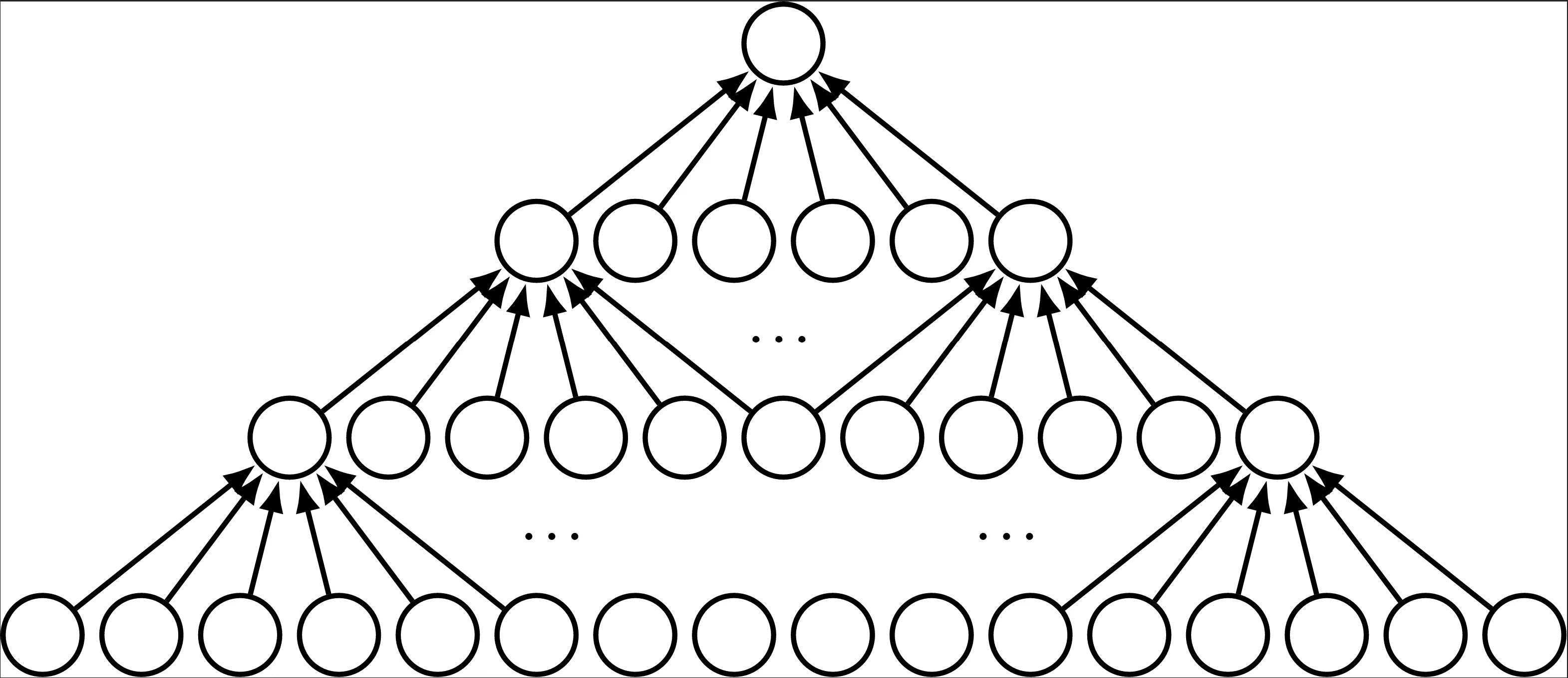
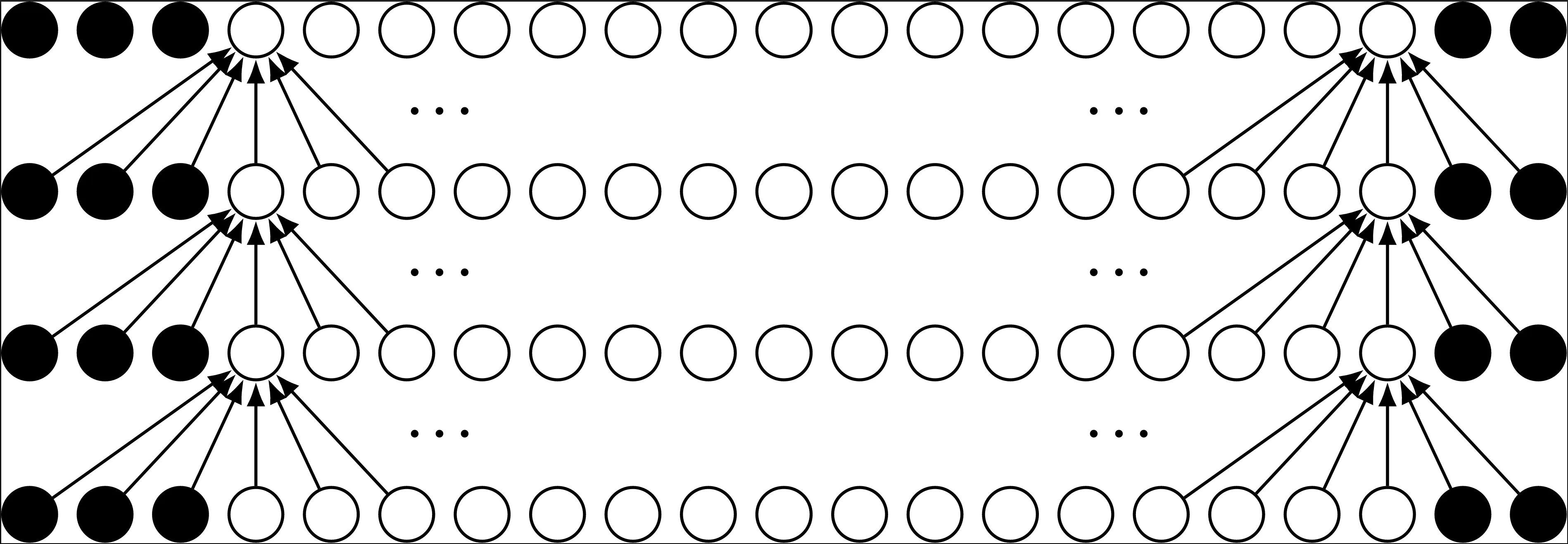
In this convolutional network, no implicit zero padding is applied. As a result, the representation decreases by five pixels at each layer. Beginning with an input of $16$ pixels, only three convolutional layers can be stacked, with the last one never actually shifting the kernel, so in practice only the first two can be considered truly convolutional. This shrinking effect can be alleviated by adopting smaller kernels, although these are less expressive, and in any case some reduction in size remains unavoidable in such an architecture.

The representation is prevented from shrinking with depth by the addition of five implicit zeros to each layer, which allows for the creation of an arbitrarily deep convolutional network.

---

Three Zero-Padding Schemes (and Convolution Modes)

It is useful to consider three special cases.

Assumptions

A $2D$ input of width $W_{\text{in}}$ is considered, together with a square kernel of width $K$, and a stride set to $S=1$.

The general formula is:

$$W_{\text{out}}=W_{\text{in}}-K+2P+1.$$

No padding $P=0$ (Valid Convolution)	Same padding, $P=\frac{K-1}{2}$, $K$ odd (Same Convolution)	Max padding $P=K-1$(Full Convolution)
The kernel is applied only where it fits entirely inside the image. In this case: $W_{\text{out}}=W_{\text{in}}-K+1$ Every output element depends on the same number of input elements, making their behavior uniform. However, the output shrinks at each layer. With large kernels, the reduction can be drastic, and stacking many layers eventually collapses the spatial dimension to $1\times 1$, after which further layers cannot be considered meaningfully convolutional.	Enough zero padding is applied to ensure that the output dimension matches the input dimension: $W_{\text{out}}=W_{\text{in}}$ In this case, the network can contain as many convolutional layers as allowed by the hardware, since the operation does not constrain the architectural possibilities for the next layer. The drawback is that pixels close to the borders affect fewer outputs than those in the center, leading to their underrepresentation in the model.	Padding is maximized so that every input element is covered in all possible positions of the kernel: $W_{\text{out}}=W_{\text{in}}+K-1$ The output grows in size, but border elements still contribute to fewer outputs than central ones. As a result, it may be hard to learn a single kernel that generalizes equally well across all positions of the feature map.

Note

In practice, the optimal amount of padding lies between valid and same.
The choice balances two competing goals: preserving spatial resolution (same) and reducing edge-related bias (valid).