Padding and Stride

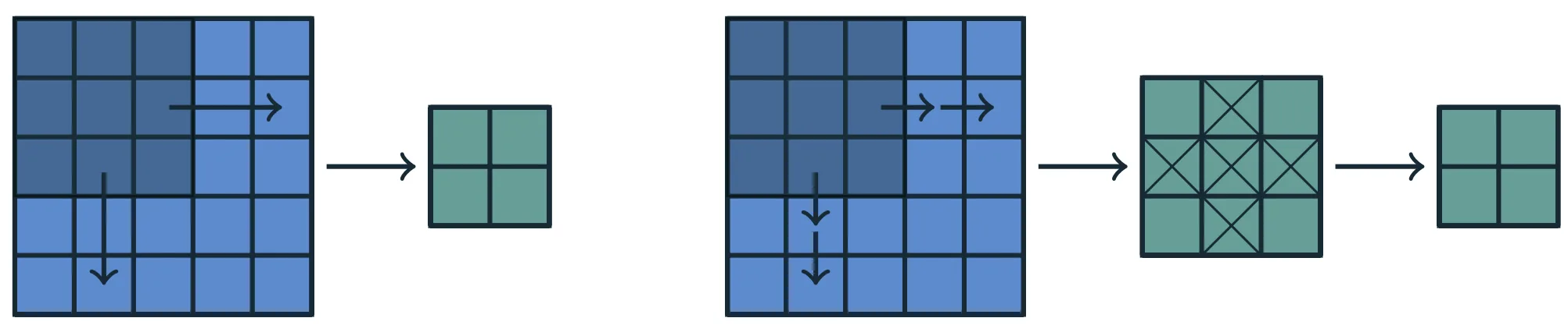
Stride

Stride

Adjacent neurons in the next layer observe translated local receptive fields in the previous layer:

• the neuron immediately to the right is sensitive to an LRF shifted one position to the right;
• the neuron immediately below is sensitive to an LRF shifted one position downward.

The amount of this translation is called the stride of the convolution.
In the standard case, the stride is 1, so the local window moves one position at a time along each spatial direction, yielding dense coverage of the domain.

This regular structure allows the convolutional layer to:

• examine the entire 2D domain systematically,
• preserve the local spatial relation between input and output,
• detect the same pattern at multiple positions.

Note

Successive neurons therefore observe different but partially overlapping regions of the previous layer, ensuring continuous coverage of the bidimensional domain.

Output-size arithmetic can be derived one axis at a time

Kernel size, padding, and stride act independently along each spatial axis.
For this reason, the derivation may focus on a single axis, such as width.
The same reasoning then applies, mutatis mutandis, to height and to any additional spatial dimension.

---

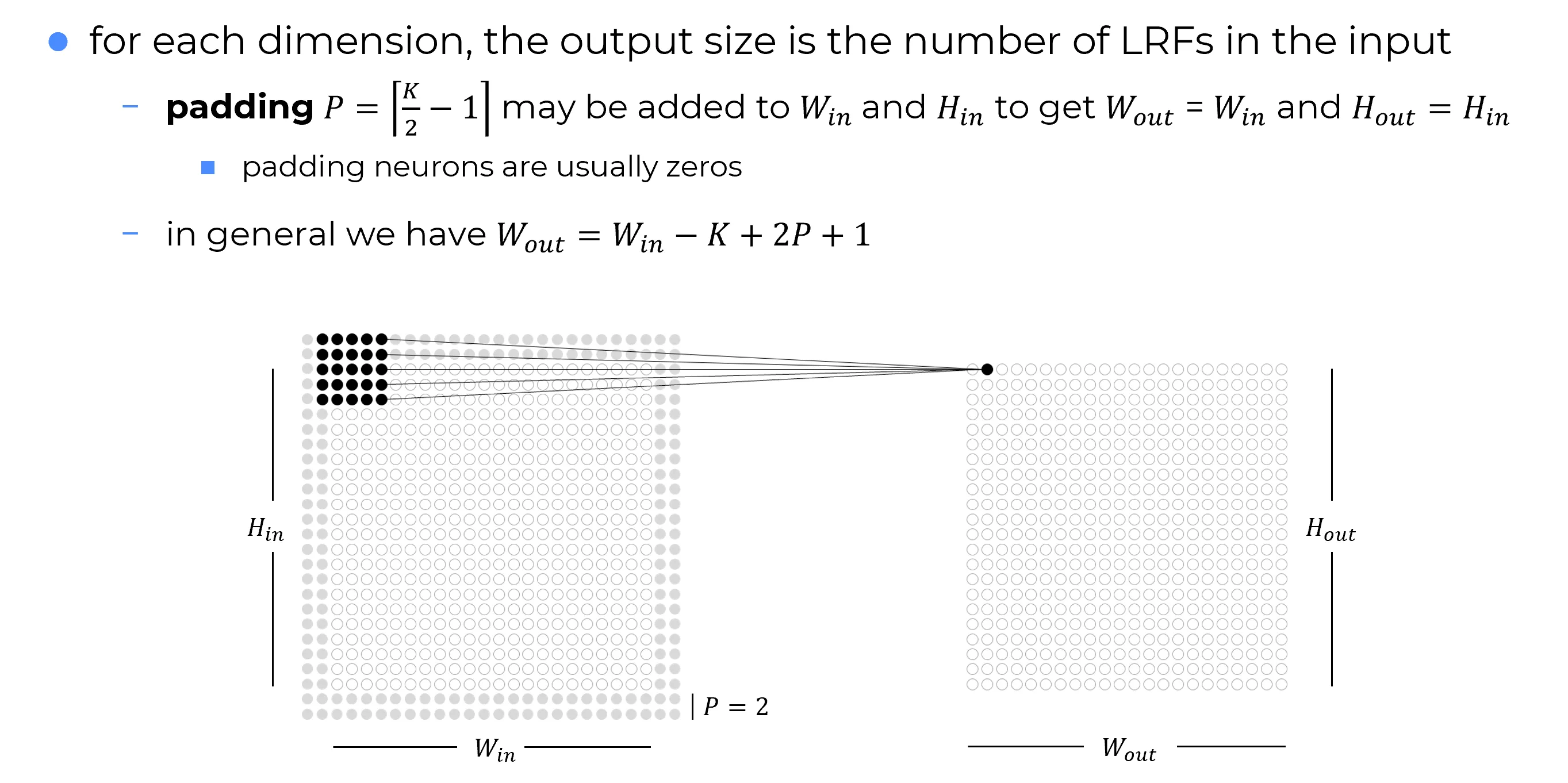
Padding

When the Local Receptive Field is shifted across the domain, a boundary problem arises that is also well known in Image Processing.

Problem

Assume a layer $\ell$ in a convolutional network under the following conditions:

• the layer input is a $2D$ matrix;
• the kernel has square shape $K\times K$;
• the stride is $S=1$;
• no extra values are added around the borders of the input.

At the boundaries of the input matrix in layer $\ell$ (which is also the output of layer $\ell -1$), the receptive field of a neuron may extend beyond the valid region, covering positions where no activations exist.
This happens because, near the edges, the center of the LRF does not have enough surrounding space to include the entire $K\times K$ window.

Even away from the borders, every convolution naturally reduces the spatial extent of the representation. Along one axis, the no-padding, stride-$1$ case gives

$$W_{\text{out}}=W_{\text{in}}-K+1,$$

so the width shrinks by $(K-1)$ positions at every layer. The full derivation of the general formula is given below.

This creates a trade-off: either very small kernels are used, or rapid reduction in spatial extent is accepted. Both scenarios limit the expressive power of the network.

Solution: Padding

A standard solution is to apply padding, i.e. to artificially extend the input domain, usually by surrounding it with additional values, most commonly zeros.
This keeps boundary receptive fields valid and, at the same time, allows the kernel size and the output dimension to be controlled more independently.

---

Zero padding ($2D$)

In the 2D case, zero padding consists of adding rows and columns of zeros around the borders of the output matrix of the previous layer, i.e. around the input to the current convolutional layer.

This ensures that every neuron in the current layer is associated with a complete and well-defined region of the previous layer, i.e. a local receptive field, even at the edges of the domain.

What does it mean to add zeros?

Zero padding effectively introduces additional positions in the previous layer whose activations are fixed to zero.
A zero activation carries no information: it represents the absence of any contribution from that location.

In this convolutional network, no implicit zero padding is applied. As a result, the representation decreases by five pixels at each layer. Beginning with an input of $16$ pixels, only three convolutional layers can be stacked, with the last one never actually shifting the kernel, so in practice only the first two can be considered truly convolutional. This shrinking effect can be alleviated by adopting smaller kernels, although these are less expressive, and in any case some reduction in size remains unavoidable in such an architecture.

The representation is prevented from shrinking with depth by the addition of five implicit zeros to each layer, which allows for the creation of an arbitrarily deep convolutional network.

---

Output Size Along One Axis

Setup

The derivation below focuses on the output size along width.
Because convolutional hyperparameters act independently along each axis, the same formulas apply to height and to any additional spatial dimension.

Stride $1$ with symmetric padding

Note

Unless stated otherwise, the initial derivation assumes stride $S=1$.

Quantities involved

Symbol	Meaning	Note
$K$	size of the local receptive field along one axis	hyperparameter
$P$	number of zero-padding values added per side	hyperparameter
$W_{\text{in}}$	size of the input along the chosen axis	inherited from input
$W_{\text{out}}$	size of the output along the same axis	quantity to be computed

Effective size after padding

Padding inserts $P$ zeros on each side of the chosen dimension.
If width is considered, $P$ values are added on the left and $P$ values on the right.

The effective size on which the local receptive field can move is therefore

$$W_{\text{eff}}=W_{\text{in}}+2P$$

In practice, the input is surrounded by zeros, turning [data] into [zeros, data, zeros] along the chosen axis.

Counting valid LRF positions

To determine $W_{\text{out}}$, the number of distinct positions in which an LRF of size $K$ fits inside the effective domain must be counted.

• The first valid LRF starts at index $0$.
• The last valid LRF must remain entirely inside the padded domain.

If an LRF of size $K$ starts at index $x$, it occupies the interval $[x,x+K-1]$.
To remain valid, its last element must not exceed the last index of the effective width:

$$x+K-1\le W_{\text{eff}}-1⟹x\le W_{\text{eff}}-K$$

Hence the maximum valid starting position is

$$x_{\text{max}}=W_{\text{eff}}-K$$

The total number of valid positions is therefore

$$W_{\text{out}}=(\text{final index}-\text{initial index})+1$$

which gives

$$W_{\text{out}}=(W_{\text{eff}}-K)-0+1=W_{\text{eff}}-K+1$$

Substituting $W_{\text{eff}}=W_{\text{in}}+2P$ yields the final result:

$$\boxed{W_{\text{out}}=W_{\text{in}}-K+2P+1}$$

By the same reasoning,

$$\boxed{H_{\text{out}}=H_{\text{in}}-K+2P+1}$$

and, in a $3D$ domain, the same argument applies to depth.

General single-axis rule

The relation

$${\text{size}}_{\text{out}}={\text{size}}_{\text{in}}-K+2P+1$$

holds along each spatial axis when stride is $1$ and dilation is not used.

General formula for stride $S$

When the stride $S$ is greater than $1$, the local receptive field jumps by $S$ positions instead of sliding by one position at a time. In that case, the number of valid positions becomes

$$\boxed{W_{\text{out}}=\lfloor \frac{W_{\text{in}}-K+2P}{S}\rfloor +1}$$

Info

Starting from index $0$ and moving in steps of $S$, the largest valid starting position is

$$x_{\text{max}}=\lfloor \frac{W_{\text{eff}}-K}{S}\rfloor$$

and the number of admissible positions is therefore $x_{\text{max}}+1$.

Applying the same reasoning to height gives

$$\boxed{H_{\text{out}}=\lfloor \frac{H_{\text{in}}-K+2P}{S}\rfloor +1}$$

and in a $3D$ domain the same formula extends to depth.

Padding that preserves spatial size

If the output size is required to match the input size along one axis, i.e.

$$W_{\text{out}}=W_{\text{in}},$$

then the stride-$1$ formula gives

$$W_{\text{in}}=W_{\text{in}}-K+2P+1$$

which simplifies to

$$2P=K-1⟹\boxed{P=\frac{K-1}{2}}$$

Kernel type	Key idea	Padding formula	Practical examples
Odd	Exact symmetric padding preserves the spatial size when stride is $1$.	$P=\frac{K-1}{2}$	$K=3\Rightarrow P=1$ $K=5\Rightarrow P=2$
Even / general	Exact size preservation is impossible with symmetric padding. A nearest symmetric choice keeps the size as close as possible.	$P=\lceil \frac{K}{2}-1\rceil =\lfloor \frac{K-1}{2}\rfloor$	$K=4\Rightarrow P=1$ $K=6\Rightarrow P=2$

The standard case: odd kernels

Since the padding $P$ must be an integer, an exact and symmetric solution exists only when $(K-1)$ is even, i.e. when the kernel size $K$ is odd.
This is one of the main reasons why odd kernels such as $3\times 3$ and $5\times 5$ dominate in practice: they have a well-defined center and support exact symmetric same-size padding when stride is $1$.

Even kernels do not preserve size exactly with symmetric padding

When the kernel size is even, exact preservation of the input size is mathematically impossible under symmetric padding and stride $1$.

For example, with $K=4$, the nearest symmetric choice is $P=\lceil 4/2-1\rceil =1$.
Substituting into the general formula gives

$$W_{\text{out}}=W_{\text{in}}-4+2(1)+1=W_{\text{in}}-1$$

so the output still shrinks by one position.
This happens because an even kernel has no unique central element, making perfect symmetric alignment impossible.

---

Three Zero-Padding Schemes (and Convolution Modes)

It is useful to distinguish three special cases.

Assumptions

A $2D$ input of width $W_{\text{in}}$ is considered, together with a square kernel of width $K$, stride $S=1$, and no dilation.

The general formula is:

$$W_{\text{out}}=W_{\text{in}}-K+2P+1.$$

No padding $P=0$ (Valid Convolution)	Same padding, $P=\frac{K-1}{2}$, $K$ odd (Same Convolution)	Max padding $P=K-1$ (Full Convolution)
The kernel is applied only where it fits entirely inside the image. In this case: $W_{\text{out}}=W_{\text{in}}-K+1$ Every output element depends on the same number of input elements, making their behavior uniform. However, the output shrinks at each layer. With large kernels, the reduction can be drastic, and stacking many layers eventually collapses the spatial dimension to $1\times 1$, after which further layers cannot be considered meaningfully convolutional.	Enough zero padding is applied to ensure that the output dimension matches the input dimension: $W_{\text{out}}=W_{\text{in}}$ In this case, the network can contain as many convolutional layers as allowed by the hardware, since the operation does not constrain the architectural possibilities for the next layer. The drawback is that pixels close to the borders affect fewer outputs than those in the center, leading to their underrepresentation in the model.	Padding is maximized so that every input element is covered in all possible positions of the kernel: $W_{\text{out}}=W_{\text{in}}+K-1$ The output grows in size, but border elements still contribute to fewer outputs than central ones. As a result, it may be hard to learn a single kernel that generalizes equally well across all positions of the feature map.

Note

In practice, the optimal amount of padding often lies between valid and same.
The choice balances two competing goals: preserving spatial resolution (same) and reducing edge-related bias (valid).