Local Receptive Field

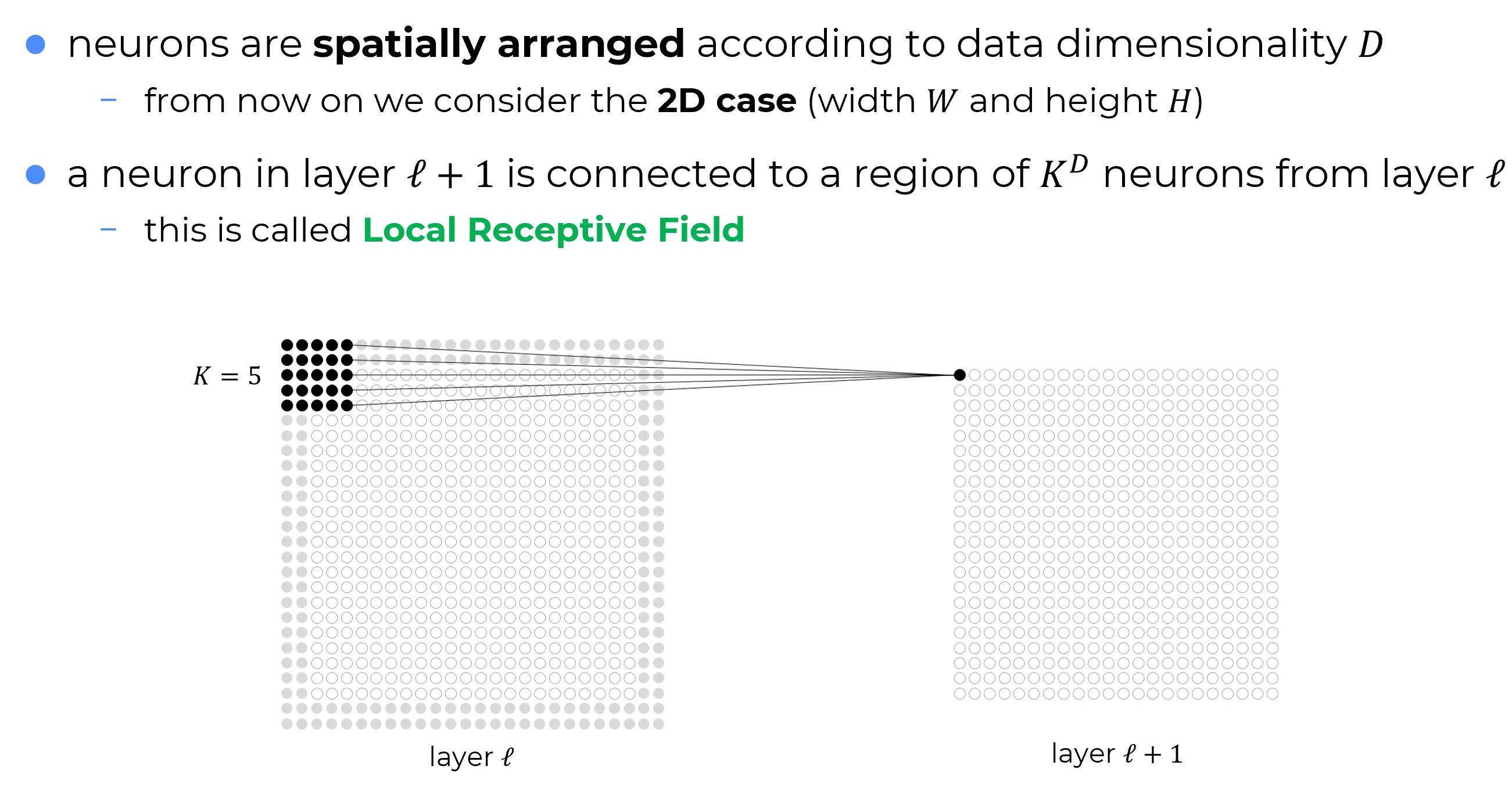
The Local Receptive Field (LRF) of a neuron within a feature map delineates the exact sub-volume of the input (i.e., the raw image or the previous input feature map) that directly drives its activation. It formally quantifies the restricted spatial context from which a single unit is able to extract information.

Etymology

• Receptive field is a term borrowed from neurophysiology: cells in the visual cortex activate only when a stimulus appears in a specific, restricted region of the retina.
• It is Local because, unlike in an MLP where each neuron of a layer is connected to all the neurons of the previous layer (i.e. fully connectivity), a CNN neuron is connected only to a small, localized topological neighborhood of the previous layer.

Let $D$ be the spatial dimensionality of the data:

• $D=1$: Signals (e.g., audio, text)
• $D=2$: Images or spectrograms
• $D=3$: Videos or volumetric data (e.g., CT, MRI scans)
• $D>3$: Multi-dimensional tensors (e.g., scientific data)

A Local Receptive Field defines a spatial window of shape $K_1\times K_2\times \cdots \times K_D$. However, it is crucial to understand that CNNs employ dense, global connectivity across the channel dimension ($C$). Therefore, the actual volume of activations from the previous layer $\ell$ to which a single neuron in layer $\ell +1$ is sensitive has the shape:

$$K_1\times K_2\times \cdots \times K_D\times C$$

The 2D Case ( $D=2$)

If the spatial window is $5\times 5$ (i.e., $K_1=K_2=5$), the neuron does not just look at a flat square:

• If the input is an RGB image ($C=3$), the neuron observes a volume of $5\times 5\times 3=75$ raw pixel values.
• If the input is a hidden layer with 64 feature maps ($C=64$), the neuron observes $5\times 5\times 64=1600$ abstract feature activations.

The concept remains the same, only the nature of the observed units (raw pixels vs. abstract features) changes moving from input layer to deeper hidden layers.

Isotropic vs. Anisotropic LRFs

If all spatial dimensions are equal ($K_1=K_2=\cdots =K_D=K$), the spatial LRF is an isotropic hypercube of size $K^D$ (e.g., $3\times 3$ in 2D).

While isotropic spatial kernels are the most common in standard CNNs, some domains benefit from anisotropic (non-square / non-cubic) LRFs:

• Text / OCR: Tall and narrow windows (e.g., $7\times 1$) capture vertical strokes efficiently.
• Audio / Spectrograms: Wider windows (e.g., $1\times 7$) capture distinct frequency bands over time.
• Medical Imaging: Anisotropic 3D kernels match the uneven physical slice spacing in CT/MRI volumes.

---

LRF vs. Dense Connectivity

Success

By restricting the neuron’s vision to a local window, CNNs directly solve the Loss of Spatial Prior inherent to Multi-Layer Perceptrons. Instead of flattening the image into a vector, which destroys the potential correlation among neighboring pixels, the local window preserves the spatial arrangement. Edges, textures, and geometric patterns remain perfectly interpretable.

	MLP Neuron	CNN Neuron
🔗Connectivity	Fully connected	Local (connected only to the LRF)
👁️ Receptive Field	Global (sees the entire flattened input)	Limited (sees only $K^D\times C$ activations in the case of an isotropic LRF)
Geometry	Destroyed (Loss of spatial prior)	Preserved (Spatial arrangement intact)

Final Remark

A neuron does not “see” the entire input, but only the local portion defined by the LRF.