Choosing a LR scheduler

Intro

Note

Choosing a learning-rate scheduler is not a secondary choice. It determines how the optimization regime changes over time:

how long the model remains in a high-learning-rate exploratory phase,

how aggressively exploitation begins,

whether training proceeds through a single decay trajectory or through multiple exploratory cycles.

For this reason, the scheduler should be chosen in relation to:

the optimizer,
the expected training length,
the degree of instability in the initial phase,
the available compute budget,
and the desired balance between exploration and exploitation.

Core principle

A learning-rate scheduler should not be selected in isolation. Its effect depends strongly on:

the optimizer used,

the total training horizon,

whether the scheduler is stepped per epoch or per iteration,

and whether the early phase of training is known to be unstable.

Conceptual map

The cleanest way to think about scheduler choice is to separate three distinct decisions:

Startup control: does the beginning of training need explicit stabilization?
Main decay geometry: how should the learning rate evolve during the bulk of training?
Trajectory strategy: should training follow one decay trajectory or several exploratory cycles?

This immediately clarifies the role of the main scheduler ingredients:

warm-up is primarily a tool for startup stabilization;
step / exponential decay and cosine annealing are mainly choices about the shape of the main decay;
restarts are a choice about whether training follows one trajectory or multiple cycles.

Important

Warm-up, cosine decay, and restarts do not all solve the same problem. A strong scheduler design is usually one in which each component has a distinct role rather than being added by habit.

It is also helpful to think of a scheduler as controlling three phases of training:

startup
main descent
late exploitation

Different scheduler families make different choices about these phases.

Scheduler family	Startup	Main descent	Late exploitation
Step / Exponential decay	Usually no special treatment	Piecewise or monotone reduction	Controlled by fixed decay pattern
Cosine annealing	Usually no special treatment unless combined with warm-up	Smooth nonlinear decay	Very gentle final exploitation
Warm-up + cosine	Explicit stabilization at the beginning	Smooth decay after warm-up	Controlled late-stage convergence
Warm-up + cosine with restarts	Explicit stabilization at the beginning	Cyclic exploration-exploitation	Multiple candidate checkpoints across cycles

This viewpoint makes scheduler choice much more concrete:

if startup instability is the problem, warm-up becomes relevant;
if abrupt milestone changes are undesirable, cosine becomes a natural choice;
if one single decay trajectory seems too restrictive, restarts become worth considering.

Start simple

In most practical projects, the scheduler search should begin with simple and well-understood policies.

Empirical starting rule

A sensible first pass is usually:

start with a simple monotone decay such as Exponential Decay;

if training is unstable, overly sensitive to milestones, or clearly benefits from a smoother transition, move to Cosine Annealing;

reserve more elaborate pipelines for cases where there is a concrete reason to need them.

This is good practice because:

simple schedules are easier to tune and diagnose,
failure modes are easier to interpret,
complexity should be added only when it solves a real problem.

Note

A more sophisticated scheduler is not automatically better. It is better only if it improves the training dynamics for the actual optimizer-model-data combination under consideration.

Startup stabilization

Startup instability

The first part of training is often qualitatively different from the rest:

gradients may be poorly calibrated,
optimizer statistics may still be inaccurate,
the model may be far from any stable basin,
large updates may be disproportionately harmful.

This is precisely the regime addressed by warm-up.

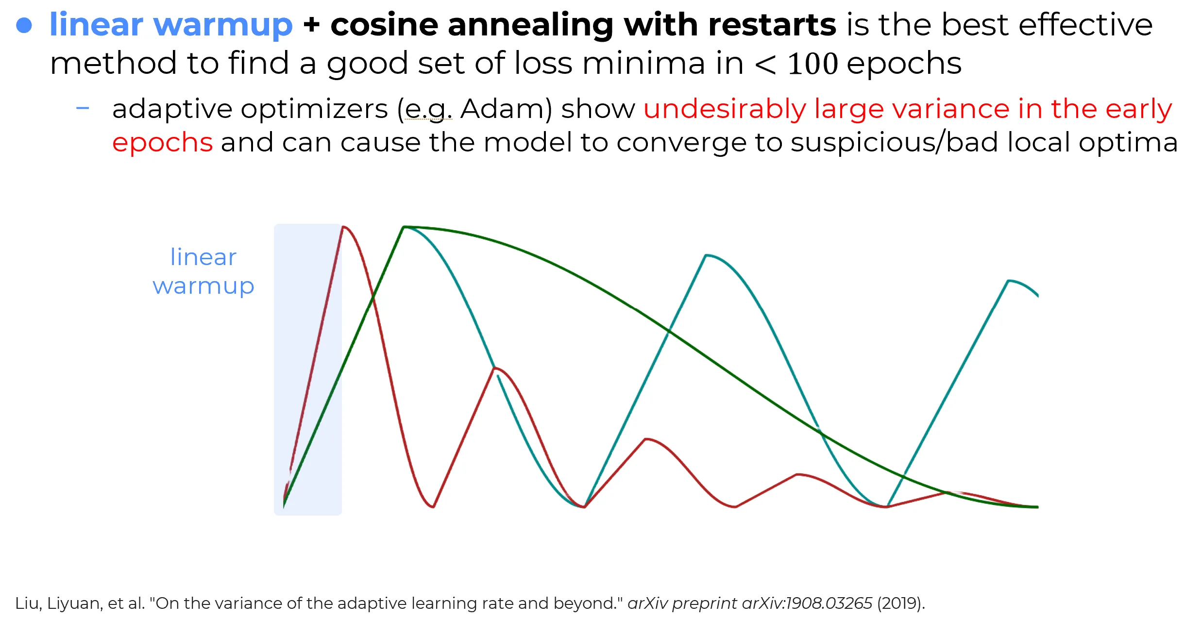
Linear warm-up

In a linear warm-up phase, the learning rate begins at a value much smaller than its target base value and then grows linearly until that target is reached.

If the warm-up lasts $T_{warm}$ steps, a simple linear warm-up can be written as

η_{t} = η_{start} + \frac{t}{T _{warm}} (η_{base} - η_{start}), 0 \leq t \leq T_{warm} .

Intuition

Warm-up does not aim to improve late-stage convergence directly. Its purpose is to prevent the optimizer from taking overly aggressive steps in the most fragile part of training.

Warm-up and adaptive optimizers

Warm-up is often discussed together with optimizers such as Adam and AdamW because, in the very first steps:

the moment estimates are still forming,
the optimization trajectory is highly sensitive,
the scale of effective updates may be unstable.

Why a high LR can be dangerous at the beginning

In adaptive optimizers, the early optimizer state may still be poorly calibrated. If the learning rate is already large during that phase, the first updates can be disproportionately aggressive, pushing the parameters into a poor region before the optimizer statistics have stabilized.

Warm-up mitigates this by ensuring that:

early updates remain conservative,
optimizer statistics have time to stabilize,
the target learning rate is reached only after the most unstable startup phase.

Note

Warm-up is not exclusive to Adam-like optimizers. It can also help in SGD-based training, especially in large-batch or otherwise sensitive regimes. However, it is particularly common in adaptive and large-scale training pipelines.

Main decay design

Monotone baseline

When no strong evidence suggests otherwise, a monotone decay schedule is often the cleanest baseline.

This includes:

step decay,
exponential decay,
other simple schedules that reduce the learning rate once or repeatedly over time.

Why begin here?

these schedules are easy to reason about,
their hyperparameters are few,
they often work surprisingly well,
and they provide a strong baseline against which more advanced schedules can be judged.

Why begin with a monotone baseline

A scheduler search should not begin from maximum complexity. It should begin from the simplest schedule that is:

technically sound,

easy to tune,

and informative when it fails.

A more advanced main schedule becomes worth considering when at least one of the following happens:

the optimization is clearly unstable at the beginning,
step-based decay is too abrupt,
training is long enough that a smoother late phase matters,
multiple exploration phases appear desirable,
the sensitivity to milestone placement is too high.

Warm-up + cosine

One of the most effective advanced pipelines is warm-up followed by cosine annealing.

This combination is often especially well suited when:

training begins in an unstable regime,
the optimizer is adaptive,
the model is large,
or the total training budget is not extremely short.

Why cosine is often effective

Once warm-up ends, the next question is how the learning rate should evolve during the main phase of training.

Cosine Annealing is compelling because it provides:

a smooth decrease,
no abrupt milestone jumps,
a naturally gentle late phase.

Its closed-form schedule over one cycle is

η_{t} = η_{m i n} + \frac{1}{2} (η_{m a x} - η_{m i n}) (1 + cos (\frac{T _{cur}}{T _{m a x}} π)) .

This makes it suitable as a main schedule after warm-up because:

training first reaches the intended working learning rate,
then decays smoothly,
then ends in a low-learning-rate exploitation regime.

Why warm-up + cosine is so often effective

The pipeline decomposes training into two phases with distinct purposes:

warm-up stabilizes the startup,

cosine decay governs the main exploration-to-exploitation trajectory.

This separation of roles is one of the main reasons the combination is so widely used.

Restart-based schedules

Warm-up + cosine + restarts

An even more aggressive strategy is to combine warm-up with cosine annealing with restarts.

The resulting training pipeline has the following structure:

a short conservative startup phase,
a first cosine exploration-to-exploitation cycle,
one or more later cycles in which the learning rate is reset and the process repeats.

This can be powerful because each cycle gives the optimizer a new opportunity to explore a different trajectory through parameter space.

High-level rationale

The idea is not that every restart must improve the model. The idea is that a single monotone schedule explores only one decay trajectory, while restarts allow several distinct exploration-exploitation phases within the same training run.

Why restart-based scheduling can help

This strategy attempts to address two different needs simultaneously:

initial stabilization, handled by warm-up;
multi-cycle exploration, handled by cosine restarts.

Thus:

warm-up protects the startup,
cosine decay controls the internal shape of each cycle,
restarts periodically reintroduce exploration.

Practical interpretation

This is best understood as an empirical high-performance recipe, not as a universally optimal theorem. It is often powerful, but it is not automatically the right choice for every training budget or every task.

Why the components are complementary

1. Warm-up stabilizes the most delicate phase

The beginning of training is often the phase in which:

optimizer statistics are least reliable,
parameter updates are most volatile,
the trajectory is most sensitive to an excessively large learning rate.

Warm-up directly targets this regime.

2. Cosine decay gives a smooth main descent

Once the optimizer has entered a more stable regime, cosine decay gives:

a smooth transition away from the high-learning-rate regime,
a longer period of substantial step sizes than an aggressively stepped decay,
and a gentle approach to low-learning-rate exploitation.

3. Restarts reintroduce exploration

If restarts are used, each cycle creates a new high-learning-rate phase. This can help produce multiple refined checkpoints and can allow the optimization trajectory to leave the neighborhood reached by the previous cycle.

4. The components have distinct roles

The reason the pipeline is compelling is that the components are not redundant:

warm-up addresses startup instability,
cosine addresses smooth decay,
restarts address single-trajectory limitations.

This clean separation of roles is what makes the pipeline conceptually strong.

Not a universal default

Note

The combination of warm-up, cosine annealing and restarts is powerful, but not always the correct default.

It may be excessive when:

the training budget is short,

startup instability is not a real issue,

a single monotone decay already works well,

the extra complexity of restart tuning is not justified.

Complexity should be earned

A sophisticated scheduler should be adopted because it solves a concrete problem:

unstable startup,

excessive sensitivity to milestones,

poor late-stage exploitation,

or the need for multiple exploratory cycles.

It should not be adopted merely because it is more elaborate.

Decision rule

The following rule is a strong practical starting point.

A robust scheduler-selection heuristic

Start with a simple monotone decay baseline.

If the early phase is unstable, add warm-up.

If milestone-based decay feels too abrupt, try cosine annealing.

If a single decay trajectory seems limiting and the compute budget allows it, consider cosine annealing with restarts.

Only keep the more complex scheduler if it yields a genuine empirical advantage.

This is a better workflow than beginning immediately with the most elaborate pipeline.

PyTorch implementation details

In PyTorch, multiple schedulers can be chained using SequentialLR.

This makes it easy to express the common pattern:

first a warm-up phase,
then a main scheduler.

Practical PyTorch caution

SequentialLR switches schedulers after a specified number of scheduler steps. Therefore, its milestones must use the same time unit as the frequency with which scheduler.step() is called. If stepping is done per epoch, the milestone counts epochs. If stepping is done per iteration, the milestone counts iterations.

Example

from torch.optim.lr_scheduler import SequentialLR, LinearLR, CosineAnnealingWarmRestarts
 
optimizer = torch.optim.Adam(model.parameters(), lr=1e-3)
 
# 1. Warm-up scheduler
# Linear growth from 0.1% of the base LR up to the full base LR in 5 scheduler steps
warmup_scheduler = LinearLR(
    optimizer,
    start_factor=1e-3,
    end_factor=1.0,
    total_iters=5,
)
 
# 2. Main scheduler
main_scheduler = CosineAnnealingWarmRestarts(
    optimizer,
    T_0=10,
    T_mult=2,
    eta_min=1e-5,
)
 
# 3. Sequential composition
# The warm-up runs for the first 5 scheduler steps, then the cosine-restart schedule begins
scheduler = SequentialLR(
    optimizer,
    schedulers=[warmup_scheduler, main_scheduler],
    milestones=[5],
)

What this example really means

The code above is correct only after the scheduler time unit has been fixed. For example:

if scheduler.step() is called once per epoch, then total_iters=5 means 5 epochs of warm-up and T_0=10 means 10 epochs in the first cosine cycle;

if scheduler.step() is called once per batch, then both quantities are measured in iterations instead.

Typical use regimes

Warm-up followed by cosine annealing is especially well suited when:

the optimizer is Adam or AdamW,
the model is large,
the startup phase is known to be sensitive,
the training horizon is long enough for the smooth decay to matter,
and one wants a schedule that is both practical and strong.

Warm-up followed by cosine annealing with restarts is especially well suited when:

the training run is long,
the compute budget allows multiple cycles,
multiple candidate checkpoints are valuable,
and one wants repeated exploration phases rather than one monotone decay.

Summary

The choice of a learning-rate scheduler should be governed by the role the scheduler must play in the training dynamics.

The most defensible strategy is:

begin with a simple monotone decay baseline,
add warm-up if startup instability is the real problem,
move to cosine annealing if a smoother main schedule is desirable,
add restarts only if the budget and the optimization behavior justify multiple exploratory cycles.

Final takeaway

A strong scheduler is not the one with the most moving parts. It is the one whose structure matches the actual needs of the training process:

stabilization at the start,

controlled decay in the middle,

and exploitation or renewed exploration later on.

Deep Learning: Zero to Hero

Explorer

Choosing a LR scheduler

Intro

Conceptual map

Start simple

Startup stabilization

Startup instability

Linear warm-up

Warm-up and adaptive optimizers

Main decay design

Monotone baseline

Warm-up + cosine

Why cosine is often effective

Restart-based schedules

Warm-up + cosine + restarts

Why restart-based scheduling can help

Why the components are complementary

Not a universal default

Decision rule

PyTorch implementation details

Example

Typical use regimes

Summary

Graph View

Table of Contents

Backlinks