The Problem of Vanishing Gradient

Among all the obstacles that historically limited the depth of neural networks, the vanishing gradient is the most consequential. It is the architectural reason that, from the late 1980s through the mid-2000s, networks deeper than $5$ to $6$ layers were practically untrainable. The deep-learning revolution of the 2010s was, in large part, the systematic resolution of this single failure mode.

The diagnosis is brief: the gradient at an early layer is a product of many partial derivatives, one per layer between that parameter and the output. A product of many factors $\le 1$ collapses to zero exponentially fast, and any small per-layer attenuator (a saturating activation, a wide pre-activation, the sheer depth of the cascade) is enough to disable learning at the network’s foundations.

The story arc

Three independent causes of small per-layer factors are addressed in turn, each with its own architectural remedy.

1. Vanishing Gradient: the diagnosis. Multiplicative chain in $\text{BP2}$, paradox of depth (first layers learn slowest), three causes previewed, link to the recurrent analogue treated in BPTT Problems.
2. Neuron saturation: cause #1. Sigmoid and tanh have $f^{\prime }(z)\approx 0$ in their tails; a saturated neuron is silent to learning, even though it still emits an output. Contrast with the loss-side fix at the output layer.
3. ReLU: remedy #1. Non-saturating activation with $f^{\prime }(z)=1$ for $z>0$. Sparsity as a feature, dying-ReLU as the side cost, domain-dependent guidance on when to use it.
4. The *LU family: refinements of ReLU. Leaky ReLU, PReLU, ELU, SELU, GELU and Swish; comparison table, selection guide, code examples. GELU and SwiGLU as the modern Transformer defaults.
5. Weights initialization: cause #2. Naive Gaussian weights make pre-activations have variance $\propto n_{\text{in}}$, saturating sigmoid neurons at step $0$. Worked example with $1000$ inputs and a PyTorch reproduction.
6. Xavier and He initialization: remedy #2. Scaling the weight variance by the inverse of the fan-in (Xavier for tanh, He for ReLU) restores unit-variance pre-activations across layers. Three independent justifications (Johnson-Lindenstrauss isometry, gain staging, edge of chaos).
7. Skip connections: remedy for the residual cause: depth itself. Even with perfect activations and initialization, a product of many factors close to $1$ accumulates error across depth. Architectural identity paths (ResNet, Highway, Transformer residual stream) give the gradient an unattenuated backward route. The same idea reappears across time as the LSTM cell state and the GRU convex-combination update.

What this section assumes and what it produces

The reader is assumed to know the backpropagation equations $\text{BP1}-\text{BP4}$ from the MLP backpropagation note and to be comfortable with elementary probability (variance of a sum of independent random variables). The output of the section is the architectural toolkit (non-saturating activations, scaled initializations, skip connections) that, combined with normalization layers treated elsewhere, makes networks of arbitrary depth trainable in practice.

---

The previous section showed how the choice of loss function can mitigate the learning slowdown that affects neural networks with saturated output neurons: a smart choice of cost (cross-entropy paired with softmax) cancels the saturating slope at the output and lets the gradient flow. That fix acts at the boundary of the network, on the layer where the loss is evaluated.

This section addresses a different failure mode that has the same end effect (parameters stop updating, training stalls) but a different cause: a slowdown that originates inside the network, in its hidden layers, and that no choice of loss function can repair. It is called the vanishing gradient, and it is the dominant reason deep neural networks were considered impractical from the late 1980s until the mid-2000s.

The mechanism in one sentence

By the chain rule, the gradient of the loss with respect to a parameter in an early layer of a deep network is the product of many partial derivatives, one per layer between that parameter and the output. If even one of those factors is close to zero, the entire product collapses, and the parameter stops receiving a meaningful learning signal.

The multiplicative pathology

A product of many factors $\le 1$ goes to zero exponentially fast in the number of factors. With $20$ factors each equal to $0.5$, the product is $\approx 10^{-6}$. With $30$ factors equal to $0.9$, the product is $\approx 0.04$. The gradient does not have to vanish at every layer for the cumulative effect to be catastrophic: a slow leak over enough layers is just as fatal as a single missing factor.

This is the structural shape of the problem. Every remedy in this section, smarter activations, smarter initializations, smarter architecture, is an attempt to keep the per-layer factors close enough to $1$ that their product stays usable across depth.

What the gradient looks like, layer by layer

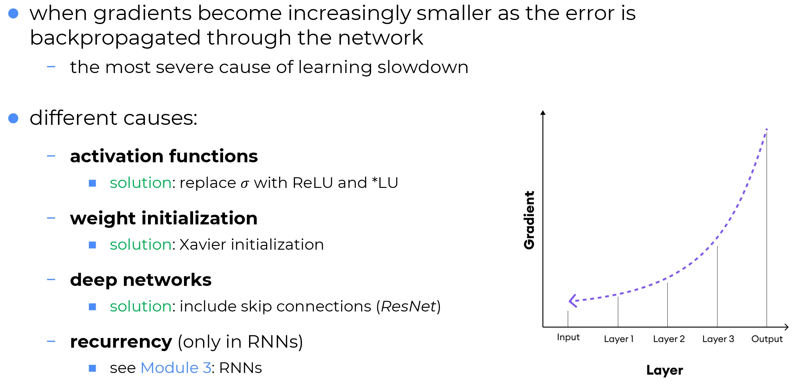
Plotting the magnitude of the gradient against layer depth in a typical deep sigmoid network produces a striking picture: the gradient is roughly of order one near the output (right side of the plot) and decays by orders of magnitude as it propagates back through the layers (right to left). By the time it reaches the early layers (left side of the plot), it is often $10^{-3}$ to $10^{-6}$ times smaller than the gradient at the output.

The consequence is a paradox of depth: the first layers, which build the low-level representations on which everything else depends, learn far more slowly than the late layers, which only refine the abstraction. The network’s foundations are precisely where the optimization signal is weakest.

Why the problem is structural

Several independent design choices conspire to make the per-layer factor small in a vanilla deep network. Each one will be analyzed in its own note, and each has a corresponding remedy.

Cause	Mechanism	Remedy	Treated in
Saturating activations	$f^{\prime }(z)\approx 0$ in the saturated regions of sigmoid and $\tanh$	non-saturating activations (ReLU and its family)	Neuron saturation, ReLU, *LU family
Bad initialization	Pre-activations have variance proportional to fan-in, pushing every neuron into saturation at step $0$	scaled initialization (Xavier, He)	Weights initialization, Xavier and He initialization
Depth itself	Even with perfect activations and initialization, the product of many Jacobians is fragile	architectural identity paths (skip connections, residual learning)	Skip connections

The three causes are independent and additive: a network can suffer from any one of them, any two, or all three at once. The deep-learning revolution of the 2010s did not pivot on a single trick but on the simultaneous adoption of all three remedies, plus normalization layers (batch / layer norm) that are orthogonal to this section.

Historical impact

In the 1980s and early 1990s, networks deeper than $5$ to $6$ layers were practically untrainable: the gradient vanished before reaching the early layers, and the experiments collapsed. Hinton, Bengio, LeCun and others (now Turing Award laureates) were aware of the problem early; the systematic fixes catalogued in this section took two decades to mature. ReLU (Glorot, Bordes and Bengio, 2011), He initialization (He et al., 2015) and residual networks (He et al., 2015) all appeared in the early 2010s and together unlocked depth on the order of hundreds of layers. The same architectural principle that fixes the recurrent vanishing-gradient problem of RNNs (a gated additive identity path through the cell state) was later identified as the same idea applied across time rather than across depth.

Mathematical setup, for reference

To make the diagnosis precise, the standard backpropagation equations are stated below without re-derivation; they are taken from the MLP backpropagation note. Let ${\mathbf{\delta }}^{\ell }$ denote the error signal at layer $\ell$, ${\mathbf{W}}^{(\ell )}$ the weight matrix between layers $\ell -1$ and $\ell$, ${\mathbf{z}}^{\ell }$ the pre-activation, and $f$ the activation function (applied component-wise). The two equations that drive the diagnosis are:

$${\mathbf{\delta }}^{\ell }=\left(\right({\mathbf{W}}^{(\ell +1)}{)}^{\top }{\mathbf{\delta }}^{(\ell +1)})\odot f^{\prime }({\mathbf{z}}^{\ell })\text{\hspace{1em}(BP2)}$$ $$\frac{\partial \mathcal{L}}{\partial w_{jk}^{\ell }}=a_k^{(\ell -1)}{\delta }_j^{\ell }\text{\hspace{1em}(BP3)}$$

Read $\text{BP2}$ as a recursion: the error at layer $\ell$ is the error at layer $\ell +1$ rotated by $({\mathbf{W}}^{(\ell +1)}{)}^{\top }$ and then gated element-wise by $f^{\prime }({\mathbf{z}}^{\ell })$. Iterating this recursion from the output layer $L$ down to layer $1$ produces, by substitution, the Jacobian product

$${\mathbf{\delta }}^1=\underset{\text{layer }1}{\underbrace{\left(\right({\mathbf{W}}^{(2)}{)}^{\top }\mathrm{diag}(f^{\prime }({\mathbf{z}}^1)))}}\cdots \underset{\text{layer }L-1}{\underbrace{\left(\right({\mathbf{W}}^{(L)}{)}^{\top }\mathrm{diag}(f^{\prime }({\mathbf{z}}^{L-1})))}}{\mathbf{\delta }}^L.$$

This is an ordered product of $L-1$ matrices, one per layer the gradient must cross. Each factor contributes one $f^{\prime }({\mathbf{z}}^{\ell })$ term, and the diagonal matrix $\mathrm{diag}(f^{\prime }({\mathbf{z}}^{\ell }))$ multiplies the cumulative product by the slope of the activation at that layer. If any single $f^{\prime }({\mathbf{z}}^{\ell })$ is small, the whole product is small, regardless of how well the other factors behave: this is the multiplicative pathology written out in full.

Equation $\text{BP3}$ then turns this attenuated ${\mathbf{\delta }}^1$ into the gradient with respect to the weights of layer $1$: multiplying by the activation $a_k^{(0)}=x_k$ of the input neuron. If ${\delta }_j^1\approx 0$, the gradient with respect to every weight feeding neuron $j$ is also approximately zero, and gradient descent has no information with which to update those weights. The early layers stop learning.

The next note zooms in on the per-layer factor $f^{\prime }({\mathbf{z}}^{\ell })$: when and why it becomes small, and what it costs the network when it does.