Skip connections

The previous notes addressed two causes of the vanishing gradient: saturating activations (fixed by ReLU and the *LU family) and badly-scaled initializations (fixed by Xavier and He). With both fixes in place, the per-layer factor in $\text{BP2}$ is close to unit magnitude in expectation.

A product of many factors close to $1$ is, however, still a product. Small deviations from unity accumulate geometrically across depth: a per-layer gain of $0.95$ becomes a cumulative gain of $0.95^{100}\approx 6\times 10^{-3}$ at depth $100$. The optimization signal that should reach the early layers still attenuates, just more slowly than under the naive initialization. Depth itself is the residual cause that no choice of activation or initialization can eliminate.

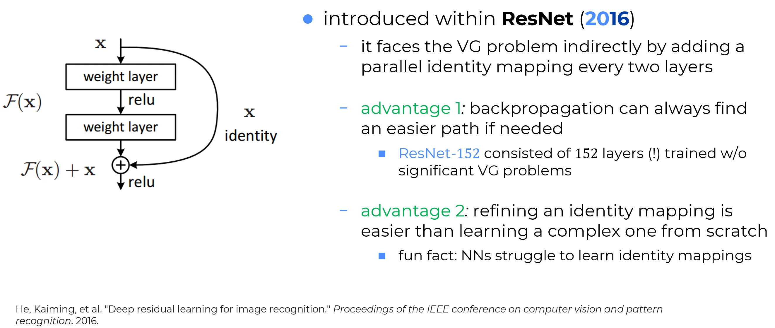
The structural remedy is to give the gradient (and the forward signal) an architectural identity path that bypasses the multiplicative cascade entirely. The construction is called a skip connection, and the family of networks built around it is the Residual Network (ResNet) of He et al. (2015), now ubiquitous in deep learning.

A diagnostic warm-up: the identity-mapping paradox

What if the network had to learn the simplest possible mapping?

Suppose a deep neural network is tasked with the trivial objective of reproducing its input as output: learn the identity $\mathbf{x}\mapsto \mathbf{x}$. Despite the triviality of the target function, a randomly initialized deep network will not approximate the identity at initialization, and gradient descent will struggle to find it by parameter updates alone.

Why learning the identity is hard

Each layer applies an affine map followed by a nonlinearity:

$${\mathbf{h}}^{(\ell )}=f({\mathbf{W}}^{(\ell )}{\mathbf{h}}^{(\ell -1)}+{\mathbf{b}}^{(\ell )}).$$

To reproduce $\mathbf{x}$ at the output of an $L$-layer network, the composition of $L$ such maps must be the identity. This requires fine-tuning all the weight matrices in concert, and the loss landscape between a random initialization and the identity solution is treacherous: the optimization signal becomes vanishingly small precisely in the regions where the early layers would need to find the identity, by the same vanishing-gradient mechanism this section is about.

The identity is as hard to learn as a complex task

For a deep neural network, “do nothing” is not an easier objective than “do something complex”. The optimizer treats both as equally demanding: each layer must individually configure its weights to participate in the global mapping, and random initialization is far from any of those configurations.

He’s reframing: residual learning

The reframing

Kaiming He and colleagues (2015) inverted the perspective: the network does not need to learn the identity explicitly. The identity can be transmitted in parallel, unchanged, alongside the layer’s transformation.

A typical residual block does three things:

1. Branch the data flow. At the input of the block, the signal splits into two paths: a main path through the layer’s affine and nonlinear transformations, and a skip path that carries the input unchanged to the block’s output.
2. Merge by addition. At the output of the block, the transformed signal is added to the original input. The addition typically takes place before the final activation, so the activation sees the combined signal.
3. Reframe the layer’s job. The layer no longer learns the entire desired output. It learns only the residual: the increment to add to the input in order to reach the desired output.

Algebraically, a vanilla layer computes

$${\mathbf{h}}^{(\ell )}=\mathcal{F}({\mathbf{h}}^{(\ell -1)};{\mathbf{\theta }}^{(\ell )}),$$

and is tasked with making $\mathcal{F}$ approximate the desired layer-to-layer mapping. A residual layer computes

$$\boxed{{\mathbf{h}}^{(\ell )}={\mathbf{h}}^{(\ell -1)}+\mathcal{F}({\mathbf{h}}^{(\ell -1)};{\mathbf{\theta }}^{(\ell )}),}$$

and is tasked with making $\mathcal{F}$ approximate the residual ${\mathbf{h}}^{(\ell )}-{\mathbf{h}}^{(\ell -1)}$. The layer’s parameters ${\mathbf{\theta }}^{(\ell )}$ are unchanged in number; only what they are asked to express has changed.

The architectural payoff

A residual layer can express the identity by setting $\mathcal{F}\equiv 0$, which is trivially achievable by driving the weights of the main path toward zero. The identity is therefore the default rather than something to be learned. Any departure from the identity is what the layer must actively encode, and that departure is by construction “small” in the sense that it is added to a signal that already carries the right shape.

With these shortcuts in place, adding depth can only help: every extra block can fall back to the identity by driving $\mathcal{F}\to 0$, so a deeper residual network is never less expressive than a shallower one, only potentially more. With the identity available for free, the network stops fighting depth and starts exploiting it.

Why residuals are easier to learn

The reframing is more than algebraic. It changes the content of the learning problem in a way that is favorable for gradient descent.

The cat-to-dog analogy

Consider transforming an image of a cat into an image of a dog. A non-residual network is asked to construct the dog image from scratch at every layer, even though the cat and the dog share most of their structure: two eyes, a nose, ears, fur. A residual network starts from the cat image and learns only what needs to change: the snout shape, the ear position, the eye colour. The shared structure rides through unchanged on the skip connection.

Most useful layer-to-layer transformations in a trained network are, in this sense, close to the identity: each layer refines the representation slightly rather than overhauling it. Learning a small residual is consistently easier than learning the full transformation, both because the target function has smaller magnitude and because the gradient with respect to the residual is independent of how close the input already is to the desired output.

Task decomposition in one line

Complex task = identity (do nothing) + residual transformation (do only what is needed).

The network no longer reinvents the input from scratch; it learns only the difference required to reach the goal. This decomposition is the conceptual core of residual learning and has reappeared in every subsequent architecture that operates at extreme depth: the LSTM cell state does the same thing across time, the GRU does it with a gated convex combination, and the Transformer residual stream does it across layers in a different form.

The gradient picture: why the highway works

The structural payoff for optimization comes from how backpropagation traverses a residual block. Consider the standard ResNet block

$${\mathbf{h}}^{(\ell )}={\mathbf{h}}^{(\ell -1)}+f({\mathbf{W}}^{(\ell )}{\mathbf{h}}^{(\ell -1)}+{\mathbf{b}}^{(\ell )}),$$

where $f$ is an element-wise nonlinearity and ${\mathbf{z}}^{(\ell )}={\mathbf{W}}^{(\ell )}{\mathbf{h}}^{(\ell -1)}+{\mathbf{b}}^{(\ell )}$ is the pre-activation of the main branch. The Jacobian of the output with respect to the input follows from differentiating the two summands separately.

The additive shortcut ${\mathbf{h}}^{(\ell -1)}$ contributes the identity, since $\partial {\mathbf{h}}^{(\ell -1)}/\partial {\mathbf{h}}^{(\ell -1)}=\mathbf{I}$. The main branch $f({\mathbf{z}}^{(\ell )})$ is the composition of a linear map and an element-wise nonlinearity, so the chain rule factors its derivative into two pieces:

• the inner map ${\mathbf{h}}^{(\ell -1)}\mapsto {\mathbf{z}}^{(\ell )}$ is linear, with Jacobian $\partial {\mathbf{z}}^{(\ell )}/\partial {\mathbf{h}}^{(\ell -1)}={\mathbf{W}}^{(\ell )}$;
• the outer map ${\mathbf{z}}^{(\ell )}\mapsto f({\mathbf{z}}^{(\ell )})$ acts coordinate by coordinate, so its Jacobian is diagonal: output coordinate $i$ depends on input coordinate $i$ alone, the off-diagonal derivatives vanish, and the $i$-th diagonal entry is $f^{\prime }(z_i^{(\ell )})$. In matrix form this is $\mathrm{diag}(f^{\prime }({\mathbf{z}}^{(\ell )}))$.

This diagonal form is worth isolating, because it reappears wherever a nonlinearity sits inside a gradient computation. Any element-wise activation has a diagonal Jacobian for the reason just given, that each output coordinate responds to its own input coordinate alone, with the slopes $f^{\prime }$ sitting on the diagonal. It is the same $\mathrm{diag}(f^{\prime }({\mathbf{z}}^{\ell }))$ that appears in every factor of the Jacobian product behind the section’s diagnosis of the vanishing gradient. The full coordinate-by-coordinate derivation is given in Backpropagation through time; in the recurrent setting the same property goes by the name no cross-coordinate mixing, and it is what holds the LSTM cell-state Jacobian diagonal across time.

Composing the outer Jacobian with the inner one, in that order, and adding the identity carried by the shortcut gives

$$\frac{\partial {\mathbf{h}}^{(\ell )}}{\partial {\mathbf{h}}^{(\ell -1)}}=\mathbf{I}+\mathrm{diag}(f^{\prime }({\mathbf{z}}^{(\ell )})){\mathbf{W}}^{(\ell )}.$$

The first term is exactly the identity, regardless of what the layer’s weights do; the second is the standard contribution of a non-residual layer.

Derivation: backward pass through a residual block

Let ${\mathbf{\delta }}^{(\ell )}=\partial \mathcal{L}/\partial {\mathbf{h}}^{(\ell )}$ denote the error signal at layer $\ell$. The residual block has two paths from ${\mathbf{h}}^{(\ell -1)}$ to ${\mathbf{h}}^{(\ell )}$:

1. The main path through $\mathcal{F}$: ${\mathbf{h}}^{(\ell -1)}\to {\mathbf{z}}^{(\ell )}={\mathbf{W}}^{(\ell )}{\mathbf{h}}^{(\ell -1)}+{\mathbf{b}}^{(\ell )}\to f({\mathbf{z}}^{(\ell )})$.
2. The skip path: ${\mathbf{h}}^{(\ell -1)}$ directly to ${\mathbf{h}}^{(\ell )}$ (the additive shortcut).

The total derivative is the sum of the contributions of the two paths. For the main path, the chain rule gives

$$\frac{\partial \mathcal{L}}{\partial {\mathbf{h}}^{(\ell -1)}}{|}_{\text{main}}=\left({\mathbf{W}}^{(\ell )}{)}^{\top }\right(f^{\prime }({\mathbf{z}}^{(\ell )})\odot {\mathbf{\delta }}^{(\ell )}).$$

For the skip path, the derivative is exactly ${\mathbf{\delta }}^{(\ell )}$ because ${\mathbf{h}}^{(\ell -1)}$ contributes to ${\mathbf{h}}^{(\ell )}$ with Jacobian $\mathbf{I}$. Adding the two,

$$\boxed{{\mathbf{\delta }}^{(\ell -1)}={\mathbf{\delta }}^{(\ell )}+\left({\mathbf{W}}^{(\ell )}{)}^{\top }\right(f^{\prime }({\mathbf{z}}^{(\ell )})\odot {\mathbf{\delta }}^{(\ell )}).}$$

The first term is the gradient passing through the skip path unchanged. The second term is the gradient passing through the main path, attenuated by $f^{\prime }$ and rotated by $({\mathbf{W}}^{(\ell )}{)}^{\top }$. Iterating across $L$ layers,

$${\mathbf{\delta }}^{(0)}=\prod _{\ell =1}^L[\mathbf{I}+({\mathbf{W}}^{(\ell )}{)}^{\top }\mathrm{diag}(f^{\prime }({\mathbf{z}}^{(\ell )}))]{\mathbf{\delta }}^{(L)}.$$

Expanding the product gives an additive sum of contributions from every possible subset of layers. The leading term, corresponding to the empty subset, is exactly ${\mathbf{\delta }}^{(L)}$: the gradient passes from output to input untouched along the all-skip path. Any vanishing happens only in the multiplicative contributions; the identity term always survives.

Two paths for the gradient

Skip connections create an alternative backward path whose product chain is much shorter than the canonical one. In a network with $L$ residual blocks, the gradient at depth $0$ is the sum of $2^L$ paths, one of which is the pure identity. As long as the identity path is structural, the optimizer is guaranteed an unattenuated route from output to input, no matter how the multiplicative paths behave.

This is the structural reason ResNets train at depths (152, 1000, and beyond) where ordinary networks of the same depth collapse.

Why the identity beats even a perfectly initialized layer

Good initialization (Xavier, He) makes each layer’s gain one in expectation: the per-layer Jacobian has unit norm on average, but it is still a random matrix scattered around that mean, so across hundreds of layers the product drifts and the early-layer gradient erodes anyway. The skip connection contributes something strictly stronger: a deterministic, exact $+\mathbf{I}$ inside the Jacobian $\mathbf{I}+\mathrm{diag}(f^{\prime })\mathbf{W}$, carrying no variance to accumulate. Initialization keeps the gain near $1$; the identity path keeps it at exactly $1$ on one route, whatever the weights do. That is the difference between “trainable up to a few dozen layers with care” and “trainable at a thousand layers by construction”.

Implementation: a residual block in PyTorch

The simplest residual block applies two convolutional layers (or two linear layers, for an MLP-style residual block) and adds the input back at the end.

import torch
import torch.nn as nn
 
class ResidualBlock(nn.Module):
    """The canonical ResNet block (for matched input/output shapes)."""
    def __init__(self, dim):
        super().__init__()
        self.fc1 = nn.Linear(dim, dim)
        self.fc2 = nn.Linear(dim, dim)
        self.relu = nn.ReLU()
 
    def forward(self, x):
        # Main path
        h = self.relu(self.fc1(x))
        h = self.fc2(h)
        # Skip path: add the input back, then apply the final activation
        return self.relu(h + x)
 
# A deep stack of residual blocks
class DeepResNet(nn.Module):
    def __init__(self, dim=128, n_blocks=100):
        super().__init__()
        self.blocks = nn.Sequential(*[ResidualBlock(dim) for _ in range(n_blocks)])
 
    def forward(self, x):
        return self.blocks(x)
 
model = DeepResNet(dim=128, n_blocks=100)
x = torch.randn(8, 128)
y = model(x)
print(y.shape)  # torch.Size([8, 128])

The block above assumes input and output have matching shapes. When the shapes differ (e.g., a CNN block that changes the number of channels or downsamples spatially), the skip path needs a projection to match the shapes:

class ProjectionResidualBlock(nn.Module):
    """Residual block with a 1x1 projection on the skip path."""
    def __init__(self, in_dim, out_dim):
        super().__init__()
        self.fc1 = nn.Linear(in_dim, out_dim)
        self.fc2 = nn.Linear(out_dim, out_dim)
        self.relu = nn.ReLU()
        # Linear projection only if shapes differ
        self.skip = nn.Linear(in_dim, out_dim) if in_dim != out_dim else nn.Identity()
 
    def forward(self, x):
        h = self.relu(self.fc1(x))
        h = self.fc2(h)
        return self.relu(h + self.skip(x))

The projection ${\mathbf{W}}_s$ on the skip path appears in $\text{BP2}$ as a transposed multiplier ${\mathbf{W}}_s^{\top }$ on the skip-path gradient. When the projection is the identity, the skip path is pure additive carry; when it is a learned linear map, the skip path still avoids the saturating activation but is no longer exactly the identity.

A pattern that recurs across architectures

The “identity highway plus learned perturbation” pattern that ResNets introduced has reappeared in every subsequent architecture that operates at extreme depth.

• The LSTM cell state is the temporal analogue: an additive carry across time instead of depth, with a learned per-coordinate decay ${\mathbf{f}}_t$ replacing the strict identity.
• The GRU is a closely related construction in which the carry weight and the new content weight are coupled by a single update gate.
• The Transformer residual stream is the same idea applied to a stack of attention and MLP sublayers: each sublayer’s output is added to the running residual, never replacing it. This is what lets modern Transformers reach depths of $100+$ layers (PaLM, GPT-4 scale) without training instability.
• Highway Networks (Srivastava et al., 2015), introduced contemporaneously with ResNets, use a gated version of the same construction with a sigmoid carry gate that adaptively trades off the skip and the transformation.

One mechanism, three timelines

The same fix appears in three independent contexts a few years apart:

year	architecture	direction of the identity path	gating
1997	LSTM	across time	per-coordinate ${\mathbf{f}}_t$
2015	GRU	across time	shared update gate ${\mathbf{z}}_t$
2015	ResNet	across depth	identity (no gating)
2015	Highway Networks	across depth	sigmoid transform gate
2017	Transformer	across depth	identity (residual stream)

The convergence is not a coincidence. All five architectures had to solve a variant of the vanishing-gradient problem, and the only architectural shape that solves it cleanly is isolate an identity path through the model, and let learned modules perturb but not replace the state on that path.

Summary

Skip connections:

• Simplify learning. The identity becomes the default behaviour rather than something the network must learn; the layers focus only on the residual increment.
• Stabilize gradient flow. Backpropagation gains an additive identity term at every block, which guarantees a non-vanishing path from the output back to the input regardless of how the multiplicative paths behave.
• Unlock depth. Networks with hundreds of layers (ResNet-152 in 2015, ResNet-1001 shortly after) become trainable, with consistent accuracy improvements from depth alone.

Closing remark

Skip connections are not a tuning trick or a regularizer; they are a structural modification that reshapes the optimization landscape. For two decades the vanishing gradient capped the usable depth of neural networks. That ceiling fell with a single structural change: an identity term inserted into every block, with the rest of the network left to learn around it. The decisive advance came from the architecture, not from any refinement of the optimizer.

Sources

Residual learning was introduced by He et al. (2015). That paper and the depth-enabling architectures around it (Highway Networks, Identity Mappings, Stochastic Depth, DenseNet) are collected in Architecture and Trainability.