Xavier and He Initialization

Solution to the learning slowdown induced by Gaussian initialization of neural-network parameters

Suppose we consider a neuron $z$ in the first hidden layer $h_1$, with $n_{in}$ input weights (see the two green layers in the previous figure).

Important

Each weight $w_{kj}^{h_1}$ is initialized so that:

$$w_{kj}^{h_1}\sim \mathcal{N}\left(0,\frac{1}{n_{\text{in}}}\right)\text{i.i.d.}j=1,\dots ,n_{\text{in}}$$

The idea is to compress the Gaussian proportionally to the number of inputs $n_{in}$: ${\sigma }_G^2=\frac{1}{n_{in}}$

In other words, the Gaussians are compressed, making it less likely that the neuron saturates. Moreover, the bias $b$ is still chosen as a Gaussian random variable with mean $0$ and standard deviation $1$.

With these choices, the net input to the neuron, $z={\sum }_j{w}_j{x}_j+b$, is again a Gaussian random variable (since Gaussian random variables are closed under linear transformations) with mean $0$, but it is much more concentrated (that is, it has smaller variance) than in the previous case.

Important

A neuron initialized in this way is much less likely to saturate and, consequently, is much less subject to learning slowdown.

Note

The bias is still initialized as $b\sim \mathcal{N}(0,1)$. This approach is acceptable, since it does not significantly increase the probability that neurons enter saturation. In reality, the way biases are initialized is not particularly critical, provided that saturation is avoided. Some even initialize all biases to $0$, relying on gradient descent to learn appropriate values afterward. However, since the choice of bias initialization has negligible impact, one initializes $b\sim \mathcal{N}(0,1)$

---

Example

Suppose, as in the previous discussion, that $500$ of the inputs are zero and $500$ are one. Then it is easy to prove that $z\sim \mathcal{N}(0,\frac{3}{2})$ (see the derivation below).

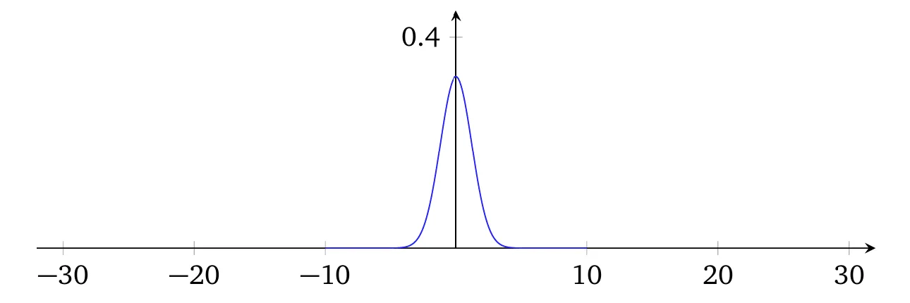
As can be observed, the distribution of the net input $z$ of the neuron under consideration is much more peaked than before, to the point that even the plot shown below does not fully convey the situation, since the vertical axis had to be rescaled with respect to the previous plot.

Rigorous proof that ${\sigma }_G^2=\frac{3}{2}$

Key assumption: The weights $w_{kj}^{h_1}$ and the bias $b$ are i.i.d. random variables.

1. Contribution of the active weights ($x_j=1$):

   • For the 500 active inputs, the partial sum is ${\sum }_{j=1}^{500}{w}_{kj}^{h_1}$.
   • Since the $w_{kj}^{h_1}\sim \mathcal{N}\left(0,\frac{1}{1000}\right)$ are i.i.d.: $$\text{Var}\left(\sum _{j=1}^{500}{w}_{kj}^{h_1}\right)=\sum _{j=1}^{500}\text{Var}(w_{kj}^{h_1})=500\cdot \left(\frac{1}{1000}\right)=\frac{1}{2}$$

2. Contribution of the bias $b\sim \mathcal{N}(0,1)$:

   $$\text{Var}(b)=1$$

3. Total variance of $z$ (by independence between weights and bias):

   $${\sigma }_G^2=\text{Var}(z)=\text{Var}\left(\sum _{j=1}^{500}{w}_{kj}^{h_1}\right)+\text{Var}(b)=\frac{1}{2}+1=\frac{3}{2}$$

The fundamental property is the additivity of variances under independence, applied both to the weights and to the bias.

---

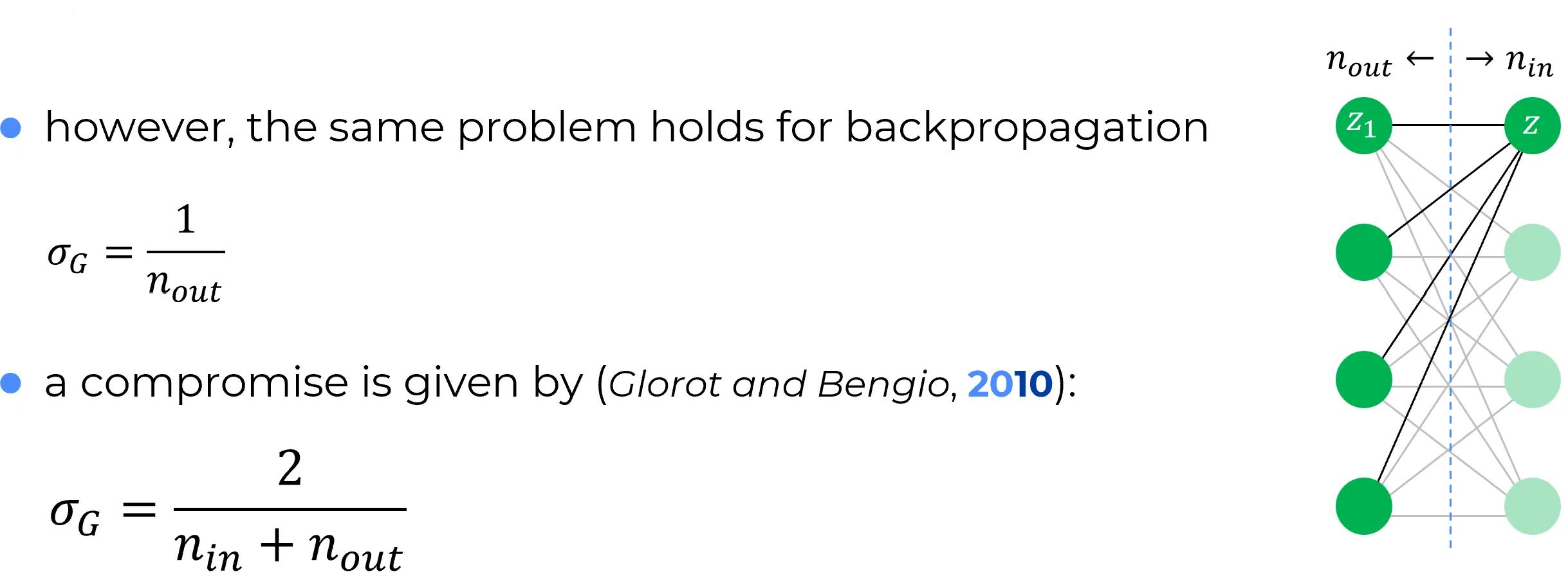
The neural network, during training, is also used from right to left by virtue of back-propagation.

It is therefore legitimate to reinterpret what was the first hidden layer as an “input” layer, and what was the input layer as the first hidden layer (see the following figure).

Following the same idea discussed above (and viewing the network from right to left), each weight associated with the output connections of neuron $z_1$ can be initialized as follows:

$$w_{kj}^{h_1}\sim \mathcal{N}\left(0,\frac{1}{n_{\text{out}}}\right)\text{i.i.d.}j=1,\dots ,n_{\text{out}}$$

where $n_{out}$ is the number of output connections (see the following note) of neuron $z_1$ in the following figure.

Note

The expression output connections of neuron $z_1$ implies reading the neural network from left to right, in feed-forward terms. Equivalently, one could use the expression incoming connections of neuron $z_1$, which instead implies reading the network from right to left, in back-propagation terms.

🔄

In the previous discussion, the analysis of the weight-initialization problem in the feedforward phase (from left to right) was separated from the analysis of the same problem in the backpropagation phase (from right to left), considering two layers in both scenarios.

However, the same reasoning could have been applied mutatis mutandis by considering a network with three layers and focusing, for example, on a neuron in the intermediate layer.

---

Xavier (Glorot-Bengio) initialization

The initialization proposed by Xavier, Glorot, and Bengio states that the weights are drawn from a normal distribution with:

$$\boxed{w_{kj}^{\ell }\sim \mathcal{N}\left(0,{\sigma }_{\text{Xavier}}^2\right),\text{i.i.d.},{\sigma }_{\text{Xavier}}^2=\frac{2}{n_{\text{in}}+n_{\text{out}}}}$$

✅ Each neuron in layer $\ell$ initializes only the weights of its incoming connections (that is, those coming from layer $\ell -1$), but the variance used for initialization also takes into account how many outgoing connections (toward layer $\ell +1$) that neuron has.

Notation used:

• $n_{\text{in}}$: number of neurons in the previous layer → connections entering the neuron
• $n_{\text{out}}$: number of neurons in the next layer → connections leaving the neuron (from its point of view)

The proposed variance ${\sigma }_{\text{Xavier}}^2$ is therefore a compromise that takes into account both the incoming and outgoing connections of a neuron.

Moreover, the biases associated with each neuron are initialized separately:

$$b_k^{\ell }\sim \mathcal{N}(0,1)$$

that is, by sampling from a standard Gaussian, independently of the weights.

---

He Initialization (Kaiming Initialization)

While Xavier (or Glorot) initialization is effective for symmetric activation functions that are linear around the origin (such as the hyperbolic tangent or the identity function), it proves inadequate for non-symmetric, non-saturating functions, particularly the Rectified Linear Unit (ReLU).

The ReLU function, defined as $f(x)=\max (0,x)$, sets all negative inputs to zero. This leads to two fundamental statistical consequences that violate Xavier’s assumptions:

1. Non-zero mean: The output of a ReLU always has a positive mean.
2. Variance halving: Assuming zero-centered inputs, ReLU “turns off” roughly half the neurons, drastically reducing the signal variance as it propagates through the network.

Therefore, using Xavier with ReLU leads to a progressive decay of variance (vanishing signal), making the training of deep networks difficult.

The Solution: He Initialization

Proposed by He et al. (2015), this initialization is specifically designed to maintain the variance of activations stable across layers in networks based on ReLU (or variants like Leaky ReLU).

Weights are drawn from a normal distribution with zero mean and a variance calibrated to compensate for the “halving” effect of ReLU:

$$\boxed{w_{kj}^{\ell }\sim \mathcal{N}\left(0,{\sigma }_{\text{He}}^2\right),\text{i.i.d.},{\sigma }_{\text{He}}^2=\frac{2}{n_{\text{in}}}}$$

Rationale behind the variance $\frac{2}{n_{in}}$

• $n_{\text{in}}$: As with Xavier, the variance is inversely proportional to the number of inputs to normalize the weighted sum.
• Factor of 2: This is the crucial adjustment for ReLU. Since ReLU zeroes out half the inputs (reducing variance by a factor of $1/2$), it is necessary to multiply the weight variance by 2 to restore the original signal level.

---

Mathematical Justification

The goal is to preserve activation variance from one layer to the next, i.e., ensuring that $\text{Var}(x^{\ell })\approx \text{Var}(x^{\ell -1})$.

Let us consider a neuron in layer $\ell$. Its pre-activation input is $y^{\ell }={\sum }_{j=1}^{n_{in}}{w}_j^{\ell }{x}_j^{\ell -1}+b^{\ell }$. We assume:

1. The weights $w$ and inputs $x$ are independent and identically distributed (i.i.d.) random variables.
2. The weights have zero mean ($E[w]=0$) and are symmetric.
3. The bias is initialized to zero ($b=0$).

The variance of the pre-activation output is:

$$\text{Var}(y^{\ell })=n_{\text{in}}\cdot \text{Var}(w^{\ell }{x}^{\ell -1})$$

Since $w$ and $x$ are independent and $E[w]=0$, the variance of the product is the product of the variances:

$$\text{Var}(y^{\ell })=n_{\text{in}}\cdot \text{Var}(w^{\ell })\cdot E[(x^{\ell -1}{)}^2]$$

Here the effect of ReLU comes into play. The input $x^{\ell -1}$ is the output of the previous layer’s ReLU ($x^{\ell -1}=\max (0,y^{\ell -1})$). If we assume that $y^{\ell -1}$ has a symmetric distribution around zero, ReLU suppresses half the values. Therefore, the second moment (signal power) is halved:

$$E[(x^{\ell -1}{)}^2]=\frac{1}{2}\text{Var}(y^{\ell -1})$$

Substituting this relation into the variance equation:

$$\text{Var}(y^{\ell })=n_{\text{in}}\cdot \text{Var}(w^{\ell })\cdot \left(\frac{1}{2}\text{Var}(y^{\ell -1})\right)$$

For the signal not to explode or vanish, we want the variance to be preserved, i.e., $\text{Var}(y^{\ell })=\text{Var}(y^{\ell -1})$. Imposing this equality:

$$\cancel{\text{Var}(y^{\ell -1})}=\frac{1}{2}{n}_{\text{in}}\text{Var}(w^{\ell })\cdot \cancel{\text{Var}(y^{\ell -1})}$$ $$1=\frac{1}{2}{n}_{\text{in}}\text{Var}(w^{\ell })⟹\text{Var}(w^{\ell })=\frac{2}{n_{\text{in}}}$$

---

Bias Initialization

Unlike the general theoretical case, when using ReLU activations it is standard practice to initialize biases to zero (or to a very small positive constant, e.g. 0.01, to avoid dead neurons, although 0 is the most common default).

$$b_k^{\ell }=0$$

Note on Biases

A Gaussian distribution is not used for biases (e.g. $b\sim \mathcal{N}(0,1)$), since it would add unnecessary variance and risk starting ReLU neurons in an “off” state (dead ReLU) if the initial value were strongly negative.