Gradient Descent (GD)

Overview

The gradient descent (GD) algorithm will be introduced by balancing intuitive reasoning with mathematical rigor.
The discussion begins with arbitrary real-valued functions $\mathcal{L}:{\mathbb{R}}^2\to \mathbb{R}$, which provide a natural geometric perspective, and is subsequently generalized to real-valued functions $\mathcal{L}:{\mathbb{R}}^n\to \mathbb{R}$. In this progression, the role of derivatives is examined, the gradient is identified as the direction of steepest ascent, and from this the update rule governing the descent process is derived.

Once the mathematical foundations are established, the focus shifts to the application of gradient descent in the training of neural networks, where the loss function $\mathcal{L}$ depends on a very large number of parameters (i.e., weights and biases). This progression, from low-dimensional intuition to high-dimensional practice, highlights both the elegance of the underlying mathematics and the challenges inherent in scaling the algorithm to modern Deep Learning.

---

Gradient Descent in ${\mathbb{R}}^2$

Let’s consider a function

$$\mathcal{L}:{\mathbb{R}}^2\to \mathbb{R},({\theta }_1,{\theta }_2)\mapsto \mathcal{L}({\theta }_1,{\theta }_2)$$

which depends on two variables, ${\theta }_1$ and ${\theta }_2$.

Goal $\mathcal{L}$ attains its global minimum.

The objective is to determine the point at which

For a simple illustrative example, the graph of such a function can be inspected directly, and the minimum identified by eye.

Note

Of course, this simplicity is somewhat artificial: the function in the example is deliberately chosen to be well-behaved so as to serve as a pedagogical aid.

A general function may depend on a large number of variables and exhibit far more complex landscapes, making visual inspection infeasible.

When Calculus Fails

One classical approach is to apply calculus: by computing derivatives, one can attempt to identify critical points where $\mathcal{L}$ achieves local extrema. While this strategy may succeed for functions of one or a few variables, it quickly becomes impractical in higher dimensions. In neural networks, for instance, the loss function typically depends on billions of weights and biases in a non trivial way, making analytical minimization via calculus essentially intractable.

Limits of 2D Intuition

Although the initial visualization in two dimensions provides useful intuition, it has its limitations. When considering functions of very high dimensionality, the two-dimensional picture inevitably breaks down. Nonetheless, cultivating multiple complementary intuitions is central to effective mathematical reasoning: one must learn when a given visualization is appropriate, when it ceases to be reliable, and how to transition between different perspectives as the problem demands.

The valley analogy

Since an analytical calculus-based minimization quickly becomes impractical in high dimensions, an alternative perspective arises from an analogy.
The function can be envisioned as defining the shape of a valley, with its graph representing the surrounding landscape.

If one imagines placing a ball somewhere on the slope, intuition suggests that it will eventually roll down toward the bottom of the valley.

Intuitive insight

This picture provides a natural metaphor for searching for a minimum: starting from an arbitrary point, the descent of the ball can be viewed as the iterative process guiding the parameters toward a lower value of the function.

Not a physical simulation

Of course, this analogy should not be interpreted literally. The objective is not to replicate the physical laws governing a real ball (e.g., friction, inertia, gravity), but rather to design an algorithmic procedure that reliably moves toward the minimum.
The ball-rolling metaphor serves as a heuristic to stimulate intuition; the actual “laws of motion” governing the descent will be chosen deliberately to ensure convergence to the bottom of the valley.

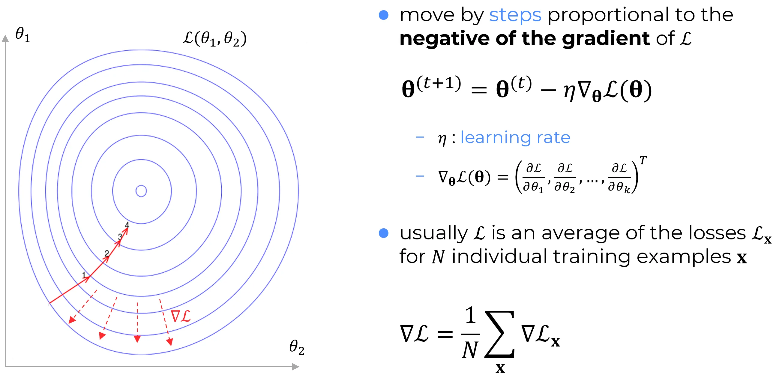
To sharpen the valley analogy, consider small displacements of the parameters.

Suppose the point $({\theta }_1,{\theta }_2)$ is perturbed by an increment $\Delta {\theta }_1$ in the ${\theta }_1$ direction and $\Delta {\theta }_2$ in the ${\theta }_2$ direction.

By a first-order Taylor approximation, the resulting change in the function is given by

$$\Delta \mathcal{L}\approx \frac{\partial \mathcal{L}}{\partial {\theta }_1}\Delta {\theta }_1+\frac{\partial \mathcal{L}}{\partial {\theta }_2}\Delta {\theta }_2\text{\hspace{1em}(1)}$$

The objective is to select the increments $\Delta {\theta }_1$ and $\Delta {\theta }_2$ such that $\Delta \mathcal{L}<0$, i.e., so that the movement corresponds to rolling down the valley toward lower values of the function.

To express this more compactly, define the vector of changes in $\mathbf{\theta }$

$$\Delta \mathbf{\theta }\equiv (\Delta {\theta }_1,\Delta {\theta }_2{)}^T,$$

where the superscript $T$ is understood to denote transposition, converting between row and column representations.

Next, the gradient of the loss function is introduced as the vector of partial derivatives:

$${\nabla }_{\mathbf{\theta }}\mathcal{L}\equiv {\left(\begin{array}{c}\frac{\partial \mathcal{L}}{\partial {\theta }_1},\frac{\partial \mathcal{L}}{\partial {\theta }_2}\end{array}\right)}^{\top }$$

This compact notation collects all first-order derivatives of $\mathcal{L}$ into a single vector.
It is worth emphasizing that $\nabla \mathcal{L}$ should be regarded as one mathematical object, the gradient vector, rather than as two separate pieces joined by a symbol.

In essence, the $\nabla$ symbol serves as notational shorthand indicating “this is the gradient of $\mathcal{L}$.”
Although in more advanced contexts $\nabla$ can be interpreted as an operator in its own right (e.g., within differential geometry), in this setting it suffices to treat $\nabla \mathcal{L}$ simply as the vector of partial derivatives defined above.

On the basis of these definitions, the expression $(1)$ for $\Delta \mathcal{L}$ can be reformulated as

$$\Delta \mathcal{L}\approx {\nabla }_{\mathbf{\theta }}\mathcal{L}\cdot \Delta \mathbf{\theta }\text{\hspace{1em}(2)}$$

This relation explains why $\nabla \mathcal{L}$ is designated as the gradient vector: it establishes a direct correspondence between variations in the parameters $\theta$ and variations in the loss $\mathcal{L}$.

Crucially, the formulation also indicates a principled way to ensure that $\Delta \mathcal{L}$ is negative.
By prescribing

$$\Delta \mathbf{\theta }=-\eta {\nabla }_{\mathbf{\theta }}\mathcal{L},$$

with $\eta >0$ denoting a small constant known as the learning rate, equation $(2)$ can be rewritten as follows:

$$\Delta \mathcal{L}\approx -\eta {\nabla }_{\mathbf{\theta }}\mathcal{L}\cdot {\nabla }_{\mathbf{\theta }}\mathcal{L}=-\eta \Vert {\nabla }_{\mathbf{\theta }}\mathcal{L}{\Vert }^2.$$

Since $\Vert {\nabla }_{\mathbf{\theta }}\mathcal{L}{\Vert }^2\ge 0$, it follows that $\Delta \mathcal{L}\le 0$.
Thus, within the limits of the linear approximation, the loss is guaranteed to decrease under this update rule.

This observation motivates the law of motion underlying the gradient descent algorithm:

$${\mathbf{\theta }}^{(t+1)}={\mathbf{\theta }}^{(t)}-\eta {\nabla }_{\mathbf{\theta }}\mathcal{L}.$$

Repeated application of this update drives the parameters downhill, progressively reducing $\mathcal{L}$, until, ideally, the process converges to a global minimum.

In summary, the gradient descent algorithm operates by repeatedly computing the gradient $\nabla \mathcal{L}$ and updating the parameters in the opposite direction, effectively moving “downhill” along the slope of the loss landscape.

It should be emphasized that this procedure does not replicate the dynamics of real physical motion. A ball rolling in a valley possesses momentum, which may carry it across the slope or even momentarily uphill before friction eventually ensures a downward trajectory. In contrast, the update rule of gradient descent prescribes an immediate step downhill at each iteration. Although simplified, this mechanism remains highly effective for locating minima.

Important

Correct functioning of the algorithm depends critically on the choice of the learning rate $\eta$.

• If $\eta$ is too large, the linear approximation used to derive the update rule no longer holds, and it is possible to obtain $\Delta \mathcal{L}>0$, which would defeat the purpose of the method.
• If $\eta$ is too small, parameter updates become negligible, causing the algorithm to converge excessively slowly.

In practice, the learning rate $\eta$ is often scheduled or adapted over time to balance these considerations, ensuring that the approximation remains valid while maintaining a reasonable rate of convergence.

Gradient Descent in higher dimensions

The discussion so far has considered the case where $\mathcal{L}$ depends on just two variables.
However, the same reasoning extends directly to functions of many variables.
Suppose that $\mathcal{L}$ is a function of $m$ parameters ${\theta }_1,\dots ,{\theta }_m$.
Then the change in $\mathcal{L}$ resulting from a small perturbation

$$\Delta \mathbf{\theta }={\left(\begin{array}{c}\Delta {\theta }_1,\dots ,\Delta {\theta }_m\end{array}\right)}^{\top }$$

is approximated by

$$\Delta \mathcal{L}\approx {\nabla }_{\mathbf{\theta }}\mathcal{L}\cdot \Delta \mathbf{\theta },$$

where the gradient is the vector of partial derivatives

$${\nabla }_{\mathbf{\theta }}\mathcal{L}\equiv {\left(\begin{array}{c}\frac{\partial \mathcal{L}}{\partial {\theta }_1},\dots ,\frac{\partial \mathcal{L}}{\partial {\theta }_m}\end{array}\right)}^{\top }.$$

As in the two-variable case, choosing

$$\Delta \mathbf{\theta }=-\eta {\nabla }_{\mathbf{\theta }}\mathcal{L},$$

with $\eta >0$ denoting the learning rate, ensures that the approximate change $\Delta \mathcal{L}$ is negative.

Thus, the parameters can be iteratively updated according to the rule

$${\mathbf{\theta }}^{(t+1)}={\mathbf{\theta }}^{(t)}-\eta {\nabla }_{\mathbf{\theta }}\mathcal{L},$$

which provides a systematic procedure for descending toward a minimum even when $\mathcal{L}$ depends on many variables.