From Perceptrons to Long-Term Memory
The history of neural networks is not a story of simply adding more layers. It is a story of making learning signals survive: first across a decision boundary, then through hidden layers, and finally across time.
The Perceptron showed that a classifier could adjust its parameters from examples. Backpropagation made hidden units reachable by gradients. LSTM changed recurrent networks by giving information and error signals a more stable path through long sequences. These are not isolated anecdotes; they are three answers to the same recurring problem:
Question
How can a network receive a training signal and preserve enough of it to learn something useful?
Abstract
This is a selective path through the history, not a complete history of neural networks. It focuses on three milestones: the Perceptron, Backpropagation, and LSTM. For other historical lines, see History of Deep Learning for the CNN lineage and History of Transformers for attention and Transformer-based models.
Neural networks before modern deep learning
Strictly speaking, these are not all “deep learning” milestones in the modern sense. They are better understood as the preconditions that made deep learning possible: trainable neurons, gradient-based learning, and mechanisms for carrying useful state across time.
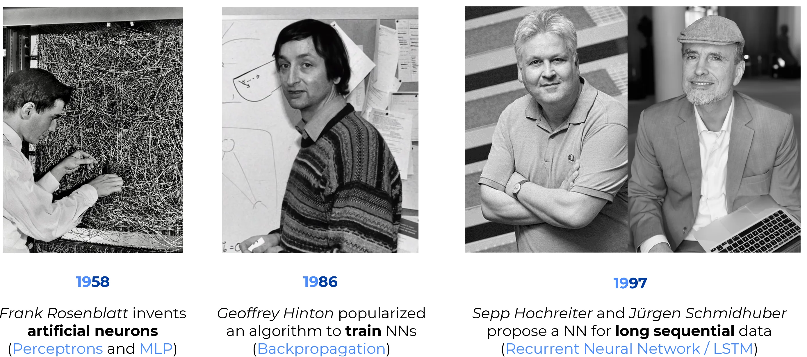
1958 – Frank Rosenblatt and the Perceptron
In the late 1950s, within the broader climate of cybernetics and early pattern recognition, Frank Rosenblatt developed the Perceptron at the Cornell Aeronautical Laboratory. It was both an engineering device for classification and a computational model inspired by biological perception.
The Perceptron is a linear threshold unit. It computes a weighted sum of the input, adds a bias term, and turns the result into a binary decision by applying a threshold.
The important idea was not that this unit was expressive. It was not. The important idea was that its parameters could be changed directly from examples: when the model made a mistake, its weights could be adjusted in the direction that would make the correct decision more likely next time. That turned classification into a learning problem. Instead of manually specifying every decision rule, the model could move its separating hyperplane in response to mistakes. Rosenblatt also demonstrated hardware feasibility through the Mark I Perceptron, an electromechanical system connected to a visual input device.
The limitation was equally important: a single-layer Perceptron can represent only linearly separable decision boundaries. This became central after Minsky and Papert’s Perceptrons (1969), which analyzed the restricted expressive power of single-layer architectures. Their critique did not prove that neural networks were useless, but it made the limits of shallow architectures hard to ignore.
Common misconception: the Perceptron critique
Minsky and Papert did not show that all neural networks were mathematically hopeless. Their analysis targeted the expressive limits of single-layer Perceptrons and related architectures.
The deeper lesson was about representation: without hidden layers or richer feature construction, many simple-looking problems remain unreachable.
Historical Anecdote: Early Hype
Public reactions to the Perceptron were far more ambitious than the mathematics justified. Contemporary press coverage framed it as a machine that might eventually acquire human-like perceptual and cognitive abilities. The scientific contribution was real; the public expectation was much larger than the model’s actual capacity.
1986 – The Popularization of Backpropagation
The next bottleneck was credit assignment inside a multi-layer network. If a hidden unit contributes indirectly to the final loss, how should its weights be changed? The output error is visible, but the responsibility of earlier layers is distributed through the whole computation.
Backpropagation answers this by applying the chain rule backward through a composed differentiable model. In a full network, this logic is organized across many layers so that shared intermediate derivatives are reused rather than recomputed. The practical routine is simple to state: run a forward pass, store the intermediate activations, run a backward pass to compute gradients, then let an optimizer update the parameters.
Info
For a dedicated introduction to the algorithm, see Introduction to Backpropagation.
This changed what could be trained. Hidden units were no longer just an architectural idea; their parameters became reachable by optimization. A network could learn internal representations rather than depend entirely on handcrafted features.
The broader methodological shift was the rise of the differentiable paradigm: design the model as a composition of differentiable operations, define a scalar loss, and let gradient-based optimization tune the parameters. CNNs, embeddings, sequence models, attention mechanisms, and modern deep learning all inherit this basic constraint.
Common misconception: 1986 was not the absolute origin
The 1986 paper by Rumelhart, Hinton, and Williams is famous because it made backpropagation visible and convincing for neural networks. It should not be described as the sole origin of the underlying mathematics.
Important precursors include:
- Seppo Linnainmaa (1970), who described reverse-mode automatic differentiation
- Paul Werbos (1974), who proposed applying these ideas to neural networks
The 1986 contribution mattered because it showed, in a clear experimental setting, that hidden layers could learn useful internal representations through gradient propagation.
1997 – Hochreiter & Schmidhuber and Long Short-Term Memory (LSTM)
Backpropagation made multi-layer networks trainable, but recurrent networks exposed a harsher version of the same problem. In a standard RNN, learning across time requires gradients to pass through many repeated transformations of the hidden state. Repeating this operation over long sequences is numerically fragile: the training signal can shrink toward zero or grow without bound, producing the vanishing and exploding gradient problem. This made long-term credit assignment difficult: the network might need information from far in the past, but the training signal could fade before reaching the relevant parameters.
Long Short-Term Memory (LSTM) changed the path through which state and error could travel. The original 1997 architecture introduced a memory cell, input gating, output gating, and the Constant Error Carousel (CEC). The core idea was to create an additive memory path where useful information could persist more stably than in a standard recurrent overwrite.
The underlying principle is not to force all memory through a single nonlinear hidden-state update. LSTM gives the model a controlled path for retaining, writing, and exposing information. This is why later LSTM variants, especially after the addition of the forget gate, became much better suited to continual input streams where the model must learn when to keep state and when to reset it.
LSTM made sequence learning more practical in tasks where distant context mattered, including speech recognition, language modeling, handwriting recognition, and machine translation. It also established a design pattern that remains important after recurrent networks: memory is not just something a model has; it is something the architecture must make trainable.
Common misconception: the forget gate came later
A common simplification is to describe the 1997 LSTM as if it already contained the modern trio of input, forget, and output gates. This is not strictly correct.
The original 1997 LSTM paper by Hochreiter and Schmidhuber introduced the memory cell, input gating, output gating, and the Constant Error Carousel. The now-standard forget gate was added later by Gers, Schmidhuber, and Cummins (2000) to allow the network to learn when to reset internal state during continual input streams.
Historical Anecdote: Slow Recognition
The core ideas behind LSTM trace back to Sepp Hochreiter’s 1991 diploma thesis. The method was not immediately treated as the default answer to sequence modeling. Over time, however, LSTMs became the standard recurrent architecture in industrial and academic sequence modeling before the rise of Transformer-based systems.
What Changed Each Time
- The Perceptron made classification learnable by adjusting a linear decision boundary from labeled examples.
- Backpropagation made hidden layers trainable by routing error signals through differentiable structure.
- LSTM made recurrent memory more trainable by stabilizing the path of information and credit assignment through time.
The Evolution of Bottlenecks
Each milestone changed the path through which learning signals could travel:
Linear classification → trainable hidden layers → long-term temporal credit assignment
Summary Table
| Year | Milestone | Why It Matters |
|---|---|---|
| 1958 | Perceptron | Established the trainable linear threshold unit and the paradigm of learning from examples. |
| 1986 | Backpropagation | Made multi-layer neural networks practically trainable through gradient-based optimization. |
| 1997 | LSTM | Gave recurrent models a more stable path for learning long-range dependencies. |
Key Take-away
Progress in neural networks often comes from changing the route through which information and error signals can travel.
- The Perceptron connected labeled mistakes to parameter updates.
- Backpropagation routed error through hidden layers.
- LSTM protected memory and credit assignment across time.
Later architectures change the same basic pathways in different ways: CNNs structure spatial computation, attention routes information by content, and Transformers remove recurrence while preserving long-range interaction. The recurring themes are still visible: parameterized computation, gradient-based learning, and architectural paths that keep useful signals alive.
Sources
The primary papers for these milestones are collected in Learning and Backpropagation, which covers the Perceptron, the Perceptrons critique, backpropagation, and LSTM together with its forget-gate refinement.