A gentle introduction to Attention

The recurrent toolkit assembled in the previous three sections (vanilla RNNs, LSTM, GRU, stacked and bidirectional variants) makes long-range sequence modelling possible, but two structural limitations of the recurrent design remain even with every fix in place:

• the forward computation is strictly sequential, so the model cannot exploit parallelism along the time axis;
• all long-range information must be routed through a finite-width hidden-state bottleneck, no matter how distant the source.

The attention mechanism addresses both limitations directly. Instead of compressing the entire history into a single hidden state at each step, attention lets the model emit a direct, learned, content-dependent pointer from any position to any other. This section builds the mechanism by iterative refinement, in the order in which the idea historically developed.

The story arc

1. A gentle introduction to Attention: the motivating case study. A simple recurrent classifier is asked to do sentiment analysis on a 44-token tweet and fails because the final hidden state has forgotten the affective word that determines the answer. Two natural fixes (concatenation, averaging) are tried and rejected. The shape of the right answer falls out from the failure analysis.
2. Soft attention: the construction. Three operations (a small scoring network, a softmax normalization, a weighted sum) produce a fixed-shape, content-dependent summary of the sequence with a parameter cost independent of sequence length. The mechanism is end-to-end differentiable, interpretable as a heat map over positions, and rich enough to fix the running example.
3. Other applications: the generalization. The same three-step pipeline applied to channels of a CNN (Squeeze-and-Excitation), spatial locations of an image (Show-Attend-and-Tell), nodes of a graph (GAT), and slots of external memory (Memory Networks, Neural Turing Machines). The abstraction that emerges is the building block of every modern attention-based architecture.

What this section is and is not

The version of attention developed here is the conceptual core, deliberately stripped to its essence: one query-free score per position, one softmax, one weighted sum.

Modern Transformer attention adds:

• query-conditional scoring,
• separate key and value projections,
• scaled dot-product scoring,
• and multiple heads.

Every one of these refinements is a strict extension of the construction in this section; none of them changes the underlying logic. Reading this section first makes the Transformer attention block in the next section read as natural rather than arbitrary.

---

Why this note exists

Modern attention mechanisms are dense with machinery (queries, keys, values, multiple heads, scaled dot products, positional encodings). Introducing all of it at once obscures the single conceptual move at the core. This note approaches the idea by iterative refinement: starts from a concrete sequence task, watches a recurrent network fail on it for a reason that is now familiar, then asks what the minimal architectural fix would look like. The fix that emerges in the next note is, structurally, the seed of everything attention has become.

What "attention" means in this section

The version of attention introduced here is the conceptual core, not the production-grade mechanism used in modern Transformers. Think of it as the “Hello, World!” of attention: enough to see why the idea works, deliberately stripped of the engineering that would distract from the principle. Modern attention is a strict refinement of this core; nothing introduced here will be discarded later.

A concrete task: binary sentiment analysis on tweets

Throughout the note, the running case study is binary sentiment classification on tweets: given a short text fragment, decide whether the predominant emotion is positive (happiness, trust, enthusiasm) or negative (anger, sadness, frustration).

On the choice of binary

Real sentiment is a multi-class, often multi-label problem: a single text fragment can simultaneously harbour a cacophony of conflicting emotions rather than a single predominant one. Restricting to binary is a deliberate simplification, made only to keep the architectural discussion uncluttered. The attention idea developed below applies unchanged to the multi-class and multi-label settings.

A worked example

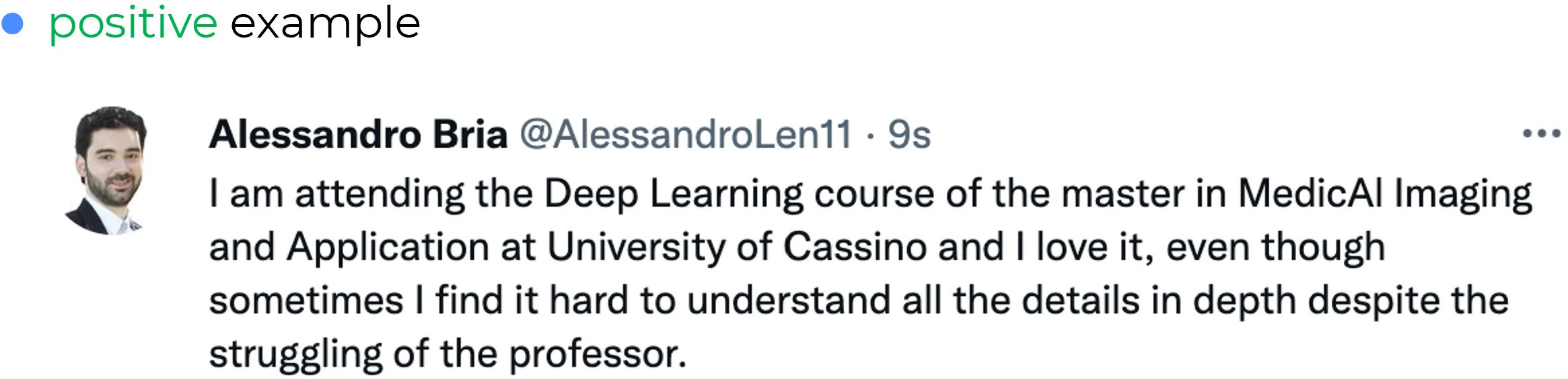
The figure below shows a tweet of positive valence, written by my professor in the voice of a student enrolled in his own course.

By visual inspection, a human reader recognizes immediately that the predominant emotion is a profound sense of affection towards Deep Learning. The word “love” sits early in the sentence; the later half (“hard”, “struggling”, “professor”) carries a more strained connotation. The overall valence is positive only because the reader integrates information from the whole sentence, weighting the affective word “love” against the surrounding context.

Goal of this section

The goal is to design a deep learning architecture capable of recognizing the predominant sentiment in a tweet, and in particular one that does not misclassify the example above. The first attempt will be a straightforward recurrent network; its failure will motivate everything that follows.

First attempt: a simple recurrent classifier

The architecture is the standard many-to-one recurrent classifier:

1. An embedding layer maps each word in the tweet (an integer index into a vocabulary) to a dense feature vector ${\mathbf{x}}_t\in {\mathbb{R}}^{d_e}$.
2. A recurrent layer (an LSTM, a GRU, or any other gated cell) consumes the embedded sequence one token at a time, producing a hidden state ${\mathbf{h}}_t\in {\mathbb{R}}^{n_{\text{neurons}}}$ at every position.
3. The final hidden state ${\mathbf{h}}_T$ (the recurrent network’s summary of the entire sentence) is fed into a fully connected sentiment-analysis head ${\text{FC}}_{\text{SA}}$ that produces the binary prediction.

Dimensions used in this note

symbol	role	shape
$w_t$	word index at position $t$ in the tweet	scalar, $t=1,\dots ,T$
${\mathbf{x}}_t$	embedded word vector	$d_e$
${\mathbf{h}}_t$	recurrent hidden state at position $t$	$n_{\text{neurons}}$
$T$	sequence length (number of tokens in the tweet)	scalar
$d_e$	embedding dimension (typically 100–300)	scalar
${\text{FC}}_{\text{SA}}$	sentiment-analysis head (fully connected)	$n_{\text{neurons}}\to 2$

The tweet in the running example has $T=44$ tokens. The recurrent state ${\mathbf{h}}_0=0$, in line with the convention used throughout these notes.

Indexing here versus in code

These theory notes index from 1: positions run $t=1,\dots ,T$, and ${\mathbf{h}}_0=0$ is reserved for the initial state. This is the convention of the attention and seq2seq literature (Bahdanau, Luong, the Transformer paper), so every formula here lines up with the papers.

Code indexes from 0. In NumPy and PyTorch, tensors start at index $0$, so in an implementation the first token is x[0], the first hidden state h[0], and the loop runs for t in range(T). The RNN code section follows this 0-based convention. The two differ only by a constant offset; nothing conceptual changes. It is the familiar gap between mathematical notation, which counts from one, and array indexing, which counts from zero.

The figures use the course-slide notation

The diagrams in this note come from the course slides and relabel two symbols: they write $n_h$ for the hidden size $n_{\text{neurons}}$ and $K$ for the sequence length $T$. Otherwise they match the text, including the colour scheme (hidden states in blue, the context vector in purple).

On embeddings

The embedding layer can be learned jointly with the architecture (its parameters are part of the network and are trained end-to-end), or it can be pretrained externally and frozen or fine-tuned.

For years the standard pretrained choice was Word2Vec (Mikolov et al., 2013); today, the best off-the-shelf contextual embeddings come from large Transformer encoders such as BERT (Devlin et al., 2019). The choice of embedding source is orthogonal to the attention question developed in this section: the same architectural arguments apply whatever produces the vectors ${\mathbf{x}}_t$.

The recurrence unrolls as ${\mathbf{h}}_t=f({\mathbf{x}}_t,{\mathbf{h}}_{t-1})$ for $t=1,\dots ,T$, with weights shared across time, exactly as in the vanilla RNN. At the end of the sentence, the final state ${\mathbf{h}}_T$ is meant to be the embedding of the whole sentence, also called the sentence representation. The classifier reads its prediction off this single vector.

"Embedding" terminology

Modern NLP uses “embedding” as a synonym for “feature vector” or “learned dense representation”.

• A word embedding is a feature vector for a word;
• a sentence embedding is a feature vector for a whole sentence;
• a contextual embedding is a feature vector for a token that depends on the surrounding text.

The word will be used in this looser sense throughout the section.

Why the simple recurrent classifier fails

The architecture above asks ${\mathbf{h}}_T$ to do a great deal of work: it must contain enough discriminative information about the entire sentence to let a single linear layer pick the correct sentiment label. For short, simple sentences this is feasible. For sequences of more than a few dozen tokens, it is not, and the reason has been discussed in depth already in BPTT Problems and Vanilla RNNs limitations.

Even gated cells (LSTM, GRU, bidirectional variants), which extend the practical horizon of useful memory by an order of magnitude over the vanilla cell, are empirically observed to forget information from the early part of the sequence when the sequence exceeds roughly 30 to 40 steps.

The architectural fix of the cell state guarantees that the gradient does not vanish along the carry path, but it does not guarantee that the network learns to actually preserve the right information across the gap; that decision is left to the gates, and the optimization signal that would teach them to do so weakens over very long sequences.

For the running example, the tweet has $T=44$ tokens. The final hidden state ${\mathbf{h}}_T$ is therefore much more strongly influenced by the second half of the sentence (the words “hard”, “struggling”, “professor”) than by the affective word “love”, which sits near the beginning. The sentiment head, reading only ${\mathbf{h}}_T$, sees mostly negative-leaning features and predicts negative, contradicting the overall valence of the tweet.

The misunderstanding pattern

The architecture has not made a small numerical error: it has structurally misunderstood the sentence, because the representation it consumes is biased toward the most recent tokens rather than the most informative ones. The single word that should dominate the decision is buried under 40 subsequent tokens of context, and no amount of widening the hidden state will recover it.

This pattern is general. In pre-Transformer NLP, recurrent encoders gave reasonable answers when the decisive evidence was locally available, and degraded sharply when the decisive evidence was several sentences earlier. The same effect bounded the quality of pre-Transformer chatbots (which lost the thread of multi-turn conversations) and pre-Transformer machine translation (which struggled with long-range agreement and word order, requiring a holistic understanding of the source sentence to translate well).

Two natural fixes, and why neither is enough

If the problem is that ${\mathbf{h}}_T$ alone forgets too much, the obvious response is to use more than just ${\mathbf{h}}_T$. Two simple constructions present themselves, and both fail for instructive reasons.

Fix 1: concatenate every hidden state

The first idea is to keep all hidden states ${\mathbf{h}}_1,{\mathbf{h}}_2,\dots ,{\mathbf{h}}_T$ and concatenate them into a single long vector $\mathbf{H}\in {\mathbb{R}}^{T\cdot n_{\text{neurons}}}$ that the sentiment head consumes:

$$\mathbf{H}=[{\mathbf{h}}_1;{\mathbf{h}}_2;\dots ;{\mathbf{h}}_T].$$

Now no information is lost: every position is exposed to the classifier. Two structural problems make this construction unusable in practice.

• The dimension scales with $T$. With $n_{\text{neurons}}=100$ and a 44-token tweet, $\mathbf{H}$ has $4400$ features. A 200-word document yields $20,000$ features. A book yields millions. The sentiment head’s weight matrix grows linearly with $T\cdot n_{\text{neurons}}$, and the number of learnable parameters of the head therefore grows linearly with sequence length.
• The dimension is not even fixed. Different tweets have different lengths, so $\mathbf{H}$ has a variable shape. A standard fully connected head cannot consume variable-shape inputs without padding to a maximum length (wasteful for short sequences and impossible for long ones).

Both pathologies share a root cause: concatenation refuses to summarize. It exposes the raw sequence to the next layer rather than producing a compact representation, and any layer that follows it inherits the burden of dealing with arbitrary-length input.

Fix 2: average every hidden state

The natural way to keep all hidden states while producing a fixed-shape summary is to average them into a single context vector $\mathbf{c}$ (the name used in the figure above):

$$\mathbf{c}=\frac{1}{T}\sum _{t=1}^T{\mathbf{h}}_t\in {\mathbb{R}}^{n_{\text{neurons}}}.$$

Now the summary has the same dimension as a single hidden state, regardless of sequence length. The sentiment head consumes a fixed-shape input; the parameter count does not depend on $T$; the architecture is well-defined.

It still gets the running example wrong. Averaging treats every position as equally informative, but the positions are not equally informative: in the tweet, the affective word “love” deserves a much heavier weight than the function word “the” or the surface word “struggling”, which is figurative rather than literal. A uniform average dilutes the salient signal among 43 unrelated tokens.

The shape of the right answer

The two failed fixes outline, between them, the constraints any acceptable mechanism must satisfy:

• fixed output shape, independent of $T$ (ruling out concatenation);
• non-uniform combination, with weights that depend on the actual content of each position (ruling out averaging);
• learnable weights, so that the network can discover which positions are salient for the task at hand;
• parameter count independent of $T$, so that the mechanism scales to arbitrary sequence lengths.

A construction satisfying all four exists, is conceptually simple, and is the subject of the next note. It is called soft attention, and it is the seed from which every modern attention mechanism grows.