First attempt

Simple RNN

With RNNs we can do many words sentences to one mapping which is the sentiment

So we can have a recurrent layer like LSTM or GRU or whatever recurrent layer, and we will feed each word of the tweet to an embedding layer which is just a layer that will translate the word to a feature vector which in turn is something that can be learnt using a fully connected layer that maps the index of the word in the dictionary to whatever is the embedding size (100, 200,300, or whatever). An embedding can be learned jointly with the architecture or it can be .. from external libraires like word2vec used for many year while now a very good embedding is BERT(Bidirectional Encoding Representation Transformer): today the best representation embedding layer is itself a transformer.

So the embedding layer transform a word into a feature vector ${\mathbf{x}}_i$ and this feature vector will be given as input to a recurrent cell and this will be done for each one of the words of the tweet. So in the figure above the time axis goes form left to right and in NLP is the direction of the text of the sentence. So the first recurrent cell outputs a certain hidden vector h_0 which is the input together with the feature vector associated to the next word of the tweet that is x_1 to the next iteration recurrent layer which shares the same weight matrixes which actually are shared through out the time axis this cell will output a hidden state vector $h_1$ which in turn will be the input of the next recurrent cell and so on until at the end of the sentence we will have the last hidden state vector $h_k$ which in our expectation should the representation of the whole sentence so h_k should be the feature vector of the whole sentence: more technically h_k should be the embedding of the whole sentence so the sentence embedding or the sentence presentation (today most used terminology in NLP is “embedding” which is just a synonym of feature representation vector).

The embedding of the whole sentence (feature representation vector h_k) is given as input to a fully connected sentiment analysis layer which will map this 1D feature vector to a 2D nuerons layer which is for binary classification evene though

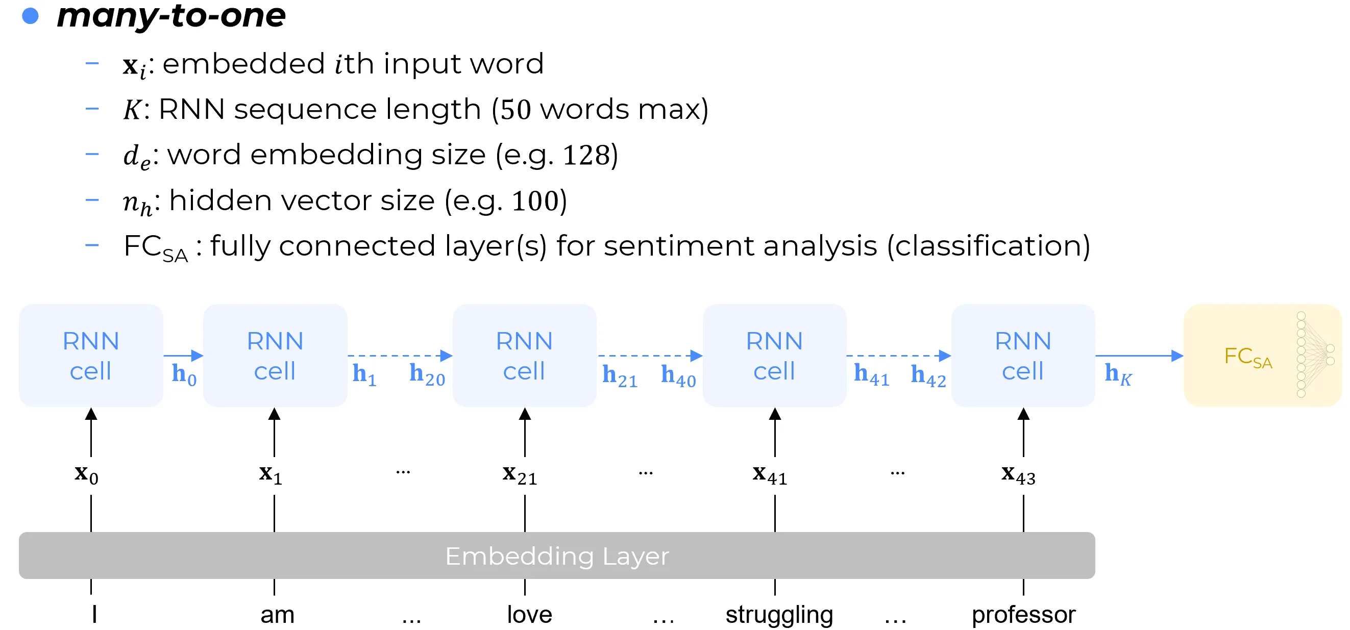
Notation:

• $x_i$ is used for inputs after the transformation of words into embeddings so x_i is the embedded input word
• k is the length of the sequence so it’s 50 word max in the old twitter: actually the tweet in question is 44 words long so i will have 44 embedding vectors form c_0 to x_43
• d_e is the dimension of the feature vector being the embedded word so each x is an emebdding of the word having size d_e whjich is the dimension of the emebdding
• the hidden vecotr size h_e is the size of the hidden state vecrtor
• FC_sa is the fully conected layer

Con le Reti Neurali Ricorrenti (RNN) è possibile realizzare una mappatura da sequenze di più parole a un’unica uscita (many-to-one mapping), la quale, nel caso in esame, corrisponde al sentimento.

Si può dunque impiegare un layer ricorrente – come ad esempio LSTM, GRU, o un qualunque altro layer di tale natura – al quale si fornirà in input ciascuna parola del tweet, previo passaggio attraverso uno strato di embedding. Quest’ultimo è essenzialmente un livello architetturale che traduce la parola in un feature vector, i cui parametri possono essere appresi tramite uno layer densamente connesso (fully connected) che mappa l’indice della parola all’interno di un vocabolario alla dimensione desiderata per l’embedding (100, 200, 300, o qualsiasi altro valore).

Un embedding può essere appreso congiuntamente all’architettura principale, oppure può essere pre-addestrato e importato da librerie esterne. Un esempio storico è Word2Vec, ampiamente utilizzato per anni, sebbene oggi rappresentazioni di qualità notevolmente superiore siano fornite da BERT (Bidirectional Encoding Representation from Transformers). Di fatto, allo stato attuale, i migliori layer di embedding e rappresentazione sono essi stessi basati su architetture Transformer.

Pertanto, il layer di embedding trasforma una parola in un feature vector ${\mathbf{x}}_i$​, e tale vettore viene fornito come input a una cella ricorrente. Questo processo viene ripetuto per ciascuna delle parole che compongono il tweet. Come illustrato nella figura di riferimento, l’asse temporale procede da sinistra verso destra, il che, nel campo dell’Elaborazione del Linguaggio Naturale (NLP), corrisponde alla direzione di lettura del testo della frase. La prima cella ricorrente produce un determinato vettore di stato nascosto ${\mathbf{h}}_0$, il quale, unitamente al feature vector ${\mathbf{x}}_1$ ​associato alla parola successiva, costituisce l’input per il layer ricorrente all’iterazione seguente. Le matrici dei pesi sono condivise lungo l’intero asse temporale. Questa cella produrrà quindi un vettore di stato nascosto ${\mathbf{h}}_1$​, che a sua volta diventerà l’input per la cella successiva, e così via, fino al raggiungimento della fine della frase.

Al termine della sequenza, si otterrà l’ultimo vettore di stato nascosto, ${\mathbf{h}}_k$​. Ci si aspetta che tale vettore costituisca la rappresentazione dell’intera frase. In termini più tecnici, ${\mathbf{h}}_k$​ dovrebbe essere il feature vector dell’intera sequenza, ovvero l’embedding dell’intera frase (sentence embedding o sentence representation).

Note

Attualmente, la terminologia più diffusa nel campo del NLP è proprio “embedding”, da intendersi come sinonimo di “vettore di rappresentazione delle caratteristiche”.

Notazione Adottata:

• Con ${\mathbf{x}}_i$​ si indica il vettore di input che si ottiene a valle della trasformazione di una parola nel suo embedding. ​ ${\mathbf{x}}_i$​ è, pertanto, la rappresentazione vettoriale della i-esima parola di input.

• $K$ denota la lunghezza della sequenza. A titolo esemplificativo, il limite massimo di parole nella precedente versione di Twitter era $50$. Poiché il tweet in esame è composto da $44$ parole, si avranno $K=44$ vettori di embedding, indicizzati da ${\mathbf{x}}_0$​ a ${\mathbf{x}}_{43}$.

• $d_e$​ indica la dimensione del vettore di embedding. Ciascun vettore xi​, rappresentante una parola, avrà dunque una dimensione pari a de​.

• $h_e$​ è la dimensione del vettore di stato nascosto (hidden state vector).

• L’acronimo ${\text{FC}}_{\text{SA}}$​ si riferisce allo strato densamente connesso (Fully Connected layer), in questo contesto impiegato per il compito di analisi del sentimento (Sentiment Analysis).