Gradient Clipping

The analysis in BPTT Problems showed that backpropagating through a deep recurrent computation can amplify gradients exponentially. When the effective scale $\gamma ={\gamma }_h{\sigma }_{\max }({\mathbf{W}}_{hh})$ exceeds $1$, the norm of the recurrent Jacobian product grows like ${\gamma }^{t-k+1}$, and the gradient of the loss with respect to the recurrent parameters can become numerically enormous. The optimizer then takes a step proportional to that gradient and overshoots wildly.

Gradient clipping is the standard defense against this failure mode. It does not change the model or the architecture; it intervenes only at the optimizer interface, rescaling the gradient whenever its norm exceeds a fixed threshold. The technique is due to Pascanu, Mikolov and Bengio (2013) and is used almost universally in RNN training.

---

Cliffs in the Loss Surface

The loss surfaces of recurrent networks have a characteristic geometric feature: cliffs. Most of the parameter space is fairly flat or gently curved, but a narrow region exists where a small change in ${\mathbf{W}}_{hh}$ causes a very large change in the loss. The reason is structural, and it can be built in four steps.

Step 1: the cell becomes linear in the right regime. The forward pass of an RNN applies the same recurrent matrix once per time step. When the hidden activations operate in the near-linear region of $\tanh$, where $\tanh (z)\approx z$ for small $z$, the cell reduces to an approximately linear map:

$${\mathbf{h}}_{t+1}\approx {\mathbf{W}}_{hh}{\mathbf{h}}_t+{\mathbf{W}}_{xh}{\mathbf{x}}_{t+1}+{\mathbf{b}}_h.$$

Step 2: iterating the linear map produces a matrix power. Substituting this approximation $T$ times along the sequence, the hidden state at the end of the sequence is

$${\mathbf{h}}_T\approx {\mathbf{W}}_{hh}^T{\mathbf{h}}_0+(\text{accumulated input-driven terms}).$$

The forward pass has effectively raised ${\mathbf{W}}_{hh}$ to the $T$-th power.

Notation

The superscript $T$ in ${\mathbf{W}}_{hh}^T$ is the sequence length, not a transpose. The transpose of a matrix $\mathbf{A}$ is written ${\mathbf{A}}^{\top }$ throughout these notes.

Step 3: a small change in ${\mathbf{W}}_{hh}$ is amplified by that power. Perturb the recurrent matrix by a tiny $\Delta {\mathbf{W}}_{hh}$. Linearising the $T$-th power around ${\mathbf{W}}_{hh}$, the induced change in ${\mathbf{h}}_T$ scales as

$$\Vert \Delta {\mathbf{h}}_T\Vert \sim \Vert {\mathbf{W}}_{hh}{\Vert }^{T-1}\Vert \Delta {\mathbf{W}}_{hh}\Vert .$$

The exponent $T-1$ is the same one that appears in the recurrent Jacobian product analysed in BPTT Problems. It is the geometric signature of the recurrent structure: an effect that happens once per step is multiplied $T$ times.

Optional: derivation of the $\Vert {\mathbf{W}}_{hh}{\Vert }^{T-1}$ scaling

Write $\mathbf{W}$ for ${\mathbf{W}}_{hh}$ for brevity. Expand $(\mathbf{W}+\Delta \mathbf{W}{)}^T$ as the product of $T$ identical factors $(\mathbf{W}+\Delta \mathbf{W})$ and keep only first-order contributions in $\Delta \mathbf{W}$. The surviving terms are exactly those in which $\Delta \mathbf{W}$ replaces $\mathbf{W}$ in one of the $T$ positions:

$$(\mathbf{W}+\Delta \mathbf{W}{)}^T={\mathbf{W}}^T+\sum _{k=0}^{T-1}{\mathbf{W}}^{T-1-k}\Delta \mathbf{W}{\mathbf{W}}^k+\mathcal{O}(\Vert \Delta \mathbf{W}{\Vert }^2).$$

If positions are numbered $0,\dots ,T-1$ from right to left, the term with $\Delta \mathbf{W}$ in position $k$ has $T-1-k$ copies of $\mathbf{W}$ on its left and $k$ on its right, hence the form ${\mathbf{W}}^{T-1-k}\Delta \mathbf{W}{\mathbf{W}}^k$.

Each of the $T$ terms is a product of $T-1$ copies of $\mathbf{W}$ and one copy of $\Delta \mathbf{W}$, so the submultiplicativity of the operator norm gives the bound

$$\Vert {\mathbf{W}}^{T-1-k}\Delta \mathbf{W}{\mathbf{W}}^k\Vert \le \Vert \mathbf{W}{\Vert }^{T-1-k}\Vert \Delta \mathbf{W}\Vert \Vert \mathbf{W}{\Vert }^k=\Vert \mathbf{W}{\Vert }^{T-1}\Vert \Delta \mathbf{W}\Vert ,$$

independent of $k$. Summing the $T$ contributions yields the worst-case bound $T\Vert \mathbf{W}{\Vert }^{T-1}\Vert \Delta \mathbf{W}\Vert$. In the exploding regime $\Vert \mathbf{W}\Vert >1$, the exponential $\Vert \mathbf{W}{\Vert }^{T-1}$ dominates the polynomial prefactor $T$ asymptotically in $T$, which is why Step 3 quotes only the exponential factor. Multiplying through by ${\mathbf{h}}_0$ gives the scaling $\Vert \Delta {\mathbf{h}}_T\Vert \sim \Vert {\mathbf{W}}_{hh}{\Vert }^{T-1}\Vert \Delta {\mathbf{W}}_{hh}\Vert$ stated above.

Step 4: the loss inherits the amplification. The loss sees the recurrent matrix only through the hidden states it produces, so the sensitivity of ${\mathbf{h}}_T$ to ${\mathbf{W}}_{hh}$ from Step 3 carries straight through to the loss. To first order, a change $\Delta {\mathbf{W}}_{hh}$ moves the loss by

$$|\Delta \mathcal{L}|\sim \Vert {\mathbf{W}}_{hh}{\Vert }^{T-1}\Vert \Delta {\mathbf{W}}_{hh}\Vert ,$$

up to a constant that does not depend on $T$ (it only measures how strongly the loss reacts to the final hidden state through the output head). The chain is the point: $\Delta {\mathbf{W}}_{hh}$ changes ${\mathbf{h}}_T$, and ${\mathbf{h}}_T$ changes the loss, and the first link carries the exponential factor $\Vert {\mathbf{W}}_{hh}{\Vert }^{T-1}$.

When $\Vert {\mathbf{W}}_{hh}\Vert >1$, that factor is enormous for a long sequence: a microscopic change in ${\mathbf{W}}_{hh}$ produces a huge change in the loss. A huge change in the loss per unit change in the parameter is, by definition, a huge gradient. This amplification is not uniform across directions. It is strongest along the direction that ${\mathbf{W}}_{hh}$ stretches the most, its dominant eigenvector, because repeated multiplication grows fastest there; perturbations along the other directions are stretched less and stay tame. The steepness is therefore concentrated in a narrow band of parameter space. That band is the cliff: a thin region where the loss surface rises almost vertically, surrounded by terrain that looks flat by comparison.

A cliff is dangerous for gradient descent because of one hidden assumption. A step $\mathbf{\theta }\leftarrow \mathbf{\theta }-\eta \nabla \mathcal{L}$ implicitly trusts that the loss stays approximately linear over the whole length of the step. The gradient is exact at the current point, but near a cliff it is so large that a step of the usual size $\eta$ travels far beyond the tiny neighborhood where the linear approximation actually holds. The update therefore overshoots the cliff and lands in an unrelated part of the loss surface, typically at a much higher loss, destroying the progress made so far.

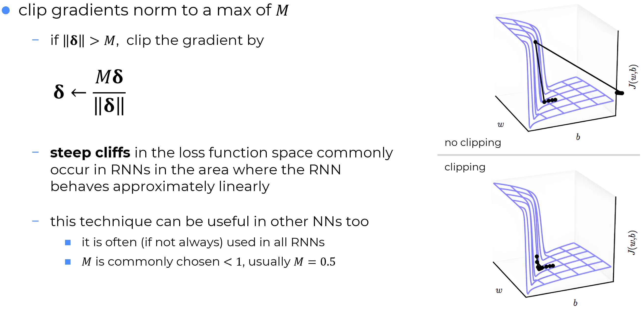
The figure makes the consequence concrete. The top panel shows a descent trajectory without clipping: the path approaches the cliff, the gradient becomes enormous along the cliff face, and the next step ejects the parameters far away from the optimum. The bottom panel shows the same trajectory with clipping: the gradient direction is preserved, but its magnitude is capped, so the step length stays bounded and the trajectory follows the cliff edge instead of being thrown off.

---

The Clipping Rule

Let $\mathbf{g}$ denote the gradient of the loss with respect to the parameters, accumulated over the mini-batch. Norm clipping replaces $\mathbf{g}$ with a rescaled version whenever its norm exceeds a fixed threshold $M$:

$$\boxed{\mathbf{g}\leftarrow \{\begin{array}{ll}\frac{M\mathbf{g}}{\Vert \mathbf{g}\Vert },& \text{if }\Vert \mathbf{g}\Vert >M,\\ \mathbf{g},& \text{otherwise.}\end{array}}$$

Two properties are worth making explicit.

• Direction is preserved. The rescaling is a positive scalar multiplication, so the clipped vector still points along $\mathbf{g}$. The optimizer is therefore still descending the loss in the same direction it would have chosen otherwise.
• Step length is capped. After clipping, $\Vert \mathbf{g}\Vert \le M$ holds by construction. The optimizer step $\eta \mathbf{g}$ is bounded by $\eta M$ regardless of how steep the cliff was.

The norm used in the formula is the Euclidean norm of the concatenation of all parameter gradients, not the norm of each layer’s gradient computed in isolation. This matters in deep networks: per-layer thresholds would not bound the total update.

Norm clipping vs value clipping

An alternative variant, value clipping, simply truncates each component of $\mathbf{g}$ into a fixed interval $[-M,M]$. It is simpler and faster to compute, but it does not preserve the gradient direction: large components are squashed disproportionately while small ones pass through unchanged. Norm clipping is the principled default and is the form implemented by torch.nn.utils.clip_grad_norm_. Value clipping is available as torch.nn.utils.clip_grad_value_ and is rarely the right choice in practice.

---

Choosing the Threshold $M$

The threshold is a hyperparameter. Typical practice in RNN training uses

$$M\in \{0.25,0.5,1.0,5.0\},$$

with $M=0.5$ a common default for vanilla and gated recurrent cells. The right value depends on three factors:

• the learning rate $\eta$, because the worst-case optimizer step is $\eta M$;
• the typical norm of unclipped gradients, which itself depends on depth, initialization, and batch size;
• the loss function and its scale (cross-entropy versus MSE, for instance).

In practice the choice is rarely critical: any $M$ in the order of $0.1$ to $10$ is usually sufficient to keep training stable, and the loss curve is fairly insensitive to the exact value as long as clipping actually triggers on the largest gradients.

Monitoring whether clipping fires

A useful diagnostic is to log the pre-clip gradient norm at every step. Three regimes are informative:

• clipping never triggers: $M$ is set too high and the technique is doing nothing;
• clipping triggers at almost every step: $M$ is set too low and the optimizer is permanently rate-limited;
• clipping triggers on the occasional spike, especially in early training: this is the healthy regime.

---

What Clipping Does Not Fix

Clipping is the canonical remedy against exploding gradients. It is not a remedy against vanishing gradients. The two failure modes have the same source (the product of recurrent Jacobians analyzed in BPTT Problems) but require entirely different interventions:

• exploding gradients are an optimizer-level problem and are fixed by a post-hoc rescaling like clipping;
• vanishing gradients are an architectural problem and are fixed by changing the cell so that the gradient has a high-bandwidth path through time. This is the role of the gates in LSTM and GRU, motivated in the limitations of vanilla RNNs.

Clipping also does nothing about the cost of unrolling a long sequence (the memory and compute that grow with $T$): that is bounded separately by the truncated and randomized schedules of BPTT Variants.

Clipping is therefore necessary but not sufficient. Modern RNN training stacks it on top of a gated cell, a gradient-friendly initialization of ${\mathbf{W}}_{hh}$, a tuned learning-rate schedule, and, for long sequences, the truncated BPTT schedule of BPTT Variants.

Beyond RNNs

The figure and the historical motivation are recurrent, but gradient clipping is also a standard component of Transformer training, where it controls the rare large-norm steps produced by the attention softmax during early epochs. Default values in modern Transformer recipes are typically $M=1.0$. The technique is, in this broader sense, less a remedy for a specific architecture than a generic safeguard against the rare optimizer step that would destroy the parameters accumulated so far.