Taxonomy of Sequential Problems

Sequential learning problems can be organized into a taxonomy by looking at the shape of the input and the shape of the output.

The symbol $x$ denotes a generic input object, while $\hat{y}$ denotes a generic model prediction. When the input is a sequence, it is written as

$${\mathbf{x}}_{1:T}=({\mathbf{x}}_1,{\mathbf{x}}_2,\dots ,{\mathbf{x}}_T).$$

Here $T$ denotes the number of elements in the sequence. In some problems this length is fixed in advance; in others it varies from example to example. Text naturally has variable length: a short review, a long article, and an entire book can all be treated as sequences, with very different values of $T$.

What counts as one sequence element?

The notation ${\mathbf{x}}_t$ emphasizes that a sequence element may be vector-valued. Scalar sequences are included as the special case where the vector has only one component.

Once the sequence elements have been converted into a fixed numerical representation, each element is written as ${\mathbf{x}}_t\in {\mathbb{R}}^d$, where $d$ is the feature dimension of one element. In text, $t$ usually indexes the position of a word or token in the sequence; in time-series data, it can index physical time. The vector ${\mathbf{x}}_t$ is the numerical representation of that element.

For a fixed numerical representation, the dimension $d$ is fixed across positions $t$. The variable quantity is the sequence length $T$, namely the number of elements appearing in the sequence.

A dataset usually contains many sequence examples. The $i$-th example may have its own length $T_i$, so sequence length can vary across the dataset.

The distinction between sequence length and element dimension should be kept explicit:

• the value $T$ counts how many ordered elements the sequence contains
• the value $d$ describes how many numerical features are used to represent one element. For a weather time series, ${\mathbf{x}}_t$ might be a single temperature value, so $d=1$. For a multivariate sensor sequence, ${\mathbf{x}}_t$ might contain temperature, humidity, pressure, and wind speed, so $d>1$.

The output has the same distinction. A model may produce a single scalar, class label, probability vector, or an entire sequence:

$${\hat{\mathbf{y}}}_{1:S}=({\hat{\mathbf{y}}}_1,{\hat{\mathbf{y}}}_2,\dots ,{\hat{\mathbf{y}}}_S).$$

Output elements can also be vectors

Each output element ${\hat{\mathbf{y}}}_s$ may also be scalar or vector-valued. A future temperature prediction may be a scalar, a sentiment classifier may output one probability vector, and a language model may output a sequence of probability vectors, one distribution over the vocabulary at each generated position.

This gives a useful taxonomy:

• in a one-to-one problem, both input and output are single objects;
• in a one-to-many problem, a single input object is mapped to an output sequence;
• in a many-to-one problem, an input sequence is mapped to a single output object;
• in a many-to-many problem, both input and output are sequences.

The many-to-many case has two important variants:

• in an aligned many-to-many problem, each input position has a corresponding output position;
• in an unaligned sequence-to-sequence problem, the output sequence may have a different length from the input sequence.

Problem type	Input	Output	Typical examples
One-to-One	A single fixed-size input	A single output	Image classification, tabular classification
One-to-Many	A single input	A sequence	Image captioning, music generation from a prompt
Many-to-One	A sequence	A single output	Sentiment analysis, activity recognition from sensor data, video classification
Many-to-Many, unaligned / Seq2Seq	A sequence	A sequence of possibly different length	Machine translation, dialogue, speech recognition, trajectory forecasting
Many-to-Many, aligned	A sequence	A sequence with corresponding positions	Part-of-speech tagging, frame-level video labeling, word-level classification

Text is represented numerically

For textual examples, raw words are first converted into numerical representations, so the model receives a sequence of vectors.

In the simplest possible representation, a vocabulary $V$ with $|V|$ words can be encoded using one-hot vectors. In that case, the feature dimension is $d=|V|$. Each word is assigned one basis vector $e_j\in {\mathbb{R}}^{|V|}$, whose entries are all zero except for a single one in the position associated with that word. A text sequence then becomes a sequence of numerical vectors: if the word at position $t$ is the $j$-th word in the vocabulary, then ${\mathbf{x}}_t=e_j$.

This representation is conceptually simple and becomes inefficient for large vocabularies, where $|V|$ can easily reach tens of thousands. Learned embeddings replace those sparse one-hot vectors with denser vectors of smaller dimension. The present taxonomy only requires the basic fact that text must be converted into numerical sequence elements before it can be processed by a sequence model.

A tiny one-hot encoding example

Consider the vocabulary

$$V=\{\text{deep},\text{learning},\text{is},\text{fun}\}.$$

Then $|V|=4$, so each word can be represented as a vector in ${\mathbb{R}}^4$:

$$\text{deep}=\left[\begin{array}{c}1\\ 0\\ 0\\ 0\end{array}\right],\text{learning}=\left[\begin{array}{c}0\\ 1\\ 0\\ 0\end{array}\right],\text{is}=\left[\begin{array}{c}0\\ 0\\ 1\\ 0\end{array}\right],\text{fun}=\left[\begin{array}{c}0\\ 0\\ 0\\ 1\end{array}\right].$$

The sentence “deep learning is fun” becomes a sequence of four 4D-vectors:

$${\mathbf{x}}_{1:4}=({\mathbf{x}}_1,{\mathbf{x}}_2,{\mathbf{x}}_3,{\mathbf{x}}_4),$$

where ${\mathbf{x}}_1$ is the vector for “deep”, ${\mathbf{x}}_2$ is the vector for “learning”, ${\mathbf{x}}_3$ is the vector for “is”, and ${\mathbf{x}}_4$ is the vector for “fun”. This example is deliberately tiny; with a real vocabulary, one-hot vectors become very high-dimensional and sparse.

---

Canonical Sequence Tasks

The following examples instantiate this taxonomy:

• lookahead prediction: a sequence prefix is used to predict one or more future elements;
• sequence classification: a full sequence is compressed into a single output, such as a sentiment label;
• sequence-to-sequence translation: an input sequence is transformed into an output sequence, possibly of different length;
• image captioning: a non-sequential input is encoded into a context vector, then decoded into a sequence.

Lookahead prediction

In lookahead prediction, the model receives a prefix of a sequence and predicts one or more future elements. Given

$$({\mathbf{x}}_1,\dots ,{\mathbf{x}}_T),$$

the desired output may be a single next element ${\hat{\mathbf{x}}}_{T+1}$ or a longer continuation

$$({\hat{\mathbf{x}}}_{T+1},\dots ,{\hat{\mathbf{x}}}_{T+\tau }).$$

The figure illustrates the prediction phase after a warmup prefix has already been processed. The model has read the input sequence up to ${\mathbf{x}}_T$, and it now produces a continuation one step at a time: first ${\hat{\mathbf{x}}}_{T+1}$, then ${\hat{\mathbf{x}}}_{T+2}$, and so on until the desired horizon $\tau$.

In text, this corresponds to next-word generation. During training, this behavior is usually learned through shifted-by-one targets: the target sequence is the input sequence shifted one step ahead, so the model learns to predict the next word at each position. During generation, the model is rolled out autoregressively: after a warmup prompt, each predicted word can be appended to the context and used to predict the following word. This autoregressive loop is the basic generation pattern behind language models.

In time-series forecasting, the same pattern is usually called autoregressive prediction: past observations are used to predict future observations. The model must maintain a representation of the prefix, because each future prediction depends on the ordered history that came before it.

If $\tau =1$, the task behaves like a many-to-one problem: a sequence prefix is mapped to one next element. If $\tau >1$, the task becomes sequence-to-sequence: a sequence prefix is mapped to a future sequence.

Sequence classification

In sequence classification, a sequence input is mapped to a single scalar, label, or probability vector. Sentiment analysis is the canonical text example: a sentence or review is processed word by word, and the model eventually produces a class distribution such as positive, negative, or neutral.

Mathematically, the input can be written as a sequence of word representations:

$${\mathbf{x}}_{1:T}=({\mathbf{x}}_1,{\mathbf{x}}_2,\dots ,{\mathbf{x}}_T).$$

The bold notation follows the convention introduced earlier: each sequence element is represented as a vector, ${\mathbf{x}}_t\in {\mathbb{R}}^d$.

A recurrent model processes the sequence one element at a time and updates a hidden state:

$${\mathbf{h}}_t=f({\mathbf{x}}_t,{\mathbf{h}}_{t-1}).$$

Sequence classification usually attaches the prediction to a summary representation of the whole sequence. In a basic recurrent model, this summary is often the final hidden state ${\mathbf{h}}_T$, which is mapped to class scores:

$$\hat{\mathbf{y}}=\mathrm{softmax}(\mathbf{W}{\mathbf{h}}_T+\mathbf{b}).$$

If there are $C$ sentiment classes, then $\hat{\mathbf{y}}\in {\mathbb{R}}^C$ is a probability vector:

$$\hat{\mathbf{y}}=({\hat{y}}_1,{\hat{y}}_2,\dots ,{\hat{y}}_C).$$

A categorical prediction can then be obtained by selecting the class with the largest probability:

$$\hat{Y}=\arg \underset{k}{\max }{\hat{y}}_k,$$

where $\hat{Y}$ is the final discrete class prediction and the scalar ${\hat{y}}_k$ denotes the $k$-th component of the probability vector $\hat{\mathbf{y}}$.

This is a many-to-one pattern: many input elements are compressed into one output object. In sentiment analysis, $\hat{\mathbf{y}}$ may be a probability vector over sentiment classes, such as positive, negative, and neutral.

Why the recurrent state matters

The recurrent state provides a mechanism for accumulating evidence as the sequence unfolds.

Machine translation

Machine translation is a sequence-to-sequence problem. The input is a sentence in one language, and the output is a sentence in another language:

$${\mathbf{x}}_{1:T}=({\mathbf{x}}_1,\dots ,{\mathbf{x}}_T)⟶{\hat{\mathbf{y}}}_{1:S}=({\hat{\mathbf{y}}}_1,\dots ,{\hat{\mathbf{y}}}_S).$$

The input length $T$ and the output length $S$ may differ. This motivates an encoder-decoder structure: the encoder processes the source sequence and produces a context representation; the decoder uses that representation to generate the target sequence one element at a time.

Beyond sequence classification

Machine translation extends sequence modeling beyond sequence classification. The model must generate a new ordered object, including its length.

Image captioning

In image captioning, the input is an image and the desired output is an ordered sentence describing that image.

The idea is to split the problem into two stages:

• a visual encoder, such as a CNN, maps the image into a latent context representation;
• a sequence decoder, such as an RNN or another autoregressive decoder, uses that context to generate the caption one word at a time.

Image captioning is a clear one-to-many problem: one input object, $x$ (i.e., an image), is mapped to an output sequence, ${\hat{\mathbf{y}}}_{1:S}$. The context vector plays a role similar to the encoder representation in machine translation, with an image encoder in place of the source-sentence encoder.

The sequence model operates on the output side. The CNN produces a compact representation of the visual content, and the decoder turns that representation into an ordered linguistic object step by step.

Object detection and sequence generation

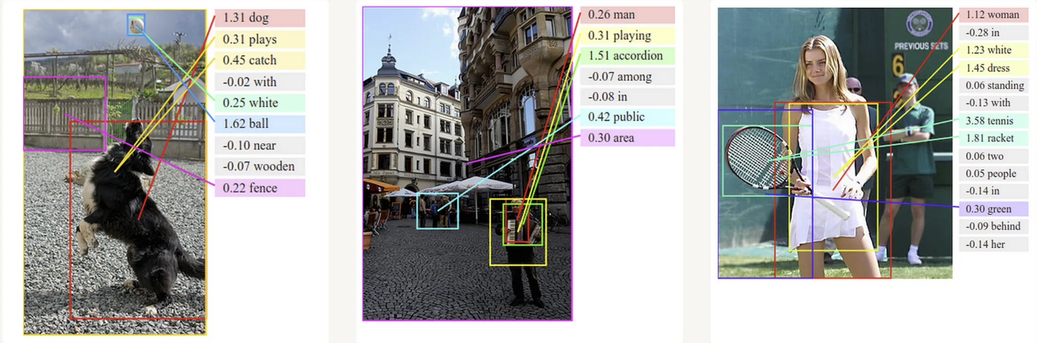
Object detection is sometimes described as one-to-many because a single image may contain multiple objects. Modern object detection is usually better viewed as structured prediction or set prediction, while image captioning is a clearer example of sequence generation.

---

Why Recurrence Becomes Natural

The examples above all point to the same underlying requirement: sequence data are ordered data. Each element must be interpreted as part of an ordered process, where meaning can depend on previous elements and on position inside the sequence.

As discussed in CNNs and MLPs limitations, standard feed-forward architectures can process sequential data after imposing a fixed input structure or relying on fixed local windows. Such approaches are useful in many cases, yet the evolving internal representation remains external to the architectural design.

Sequence modeling suggests a more natural principle: process the sequence one element at a time while carrying forward information extracted from the previous elements. This requires an internal state that evolves across positions.

Recurrence fills this conceptual gap. A recurrent model applies the same computational unit repeatedly across the sequence, updating a hidden state at each step. In this way, the forward computation itself becomes organized along the sequence dimension.

This leads naturally to Recurrent Neural Networks (RNNs), the first major neural architecture explicitly designed around sequential computation. The simplest recurrent cell is formalized in Vanilla RNN.