Learning rate scheduling

1. The complementary axis to adaptive optimization

The notes on AdaGrad, RMSProp, Adam and AdamW discuss optimizers that rescale the update coordinate by coordinate using running gradient statistics. Even after that rescaling, however, a global base learning rate $\eta$ still remains: the adaptive denominator changes the relative step size between parameters, but the overall magnitude is set by the optimizer’s lr argument.

What learning-rate scheduling is

Learning-rate scheduling is the deliberate modification of this global base learning rate over the course of training. Its purpose is to shape the optimization dynamics differently at different stages of training, with shrinking the step size being only one part of that.

The two mechanisms are complementary, not redundant:

mechanism	controls	varies along	scope
adaptive optimizer (Adam, RMSProp, etc.)	effective step size per parameter	parameter axis	within a single step
learning-rate scheduler	base learning rate ${\eta }_t$ per step	time axis	across the training run

A complete pipeline typically uses both: an adaptive optimizer to handle heterogeneous gradient scales across parameters, and a scheduler to handle the evolving needs of the training process across time.

2. Why a constant learning rate is a poor compromise

The optimization problem faced at the beginning of training is not the same as the one faced near the end.

Early in training, the model is far from any well-formed basin, gradients may be poorly calibrated, and large steps are useful for rapid progress and broad exploration. Late in training, the model already lies in a promising region, and optimization becomes sensitive to overshooting; finer steps matter more than aggressive motion.

A constant learning rate is forced to compromise between these two regimes:

• if it is chosen large enough to be useful early, it tends to be too large at the end (the optimizer keeps oscillating around the minimum it should be settling into);
• if it is chosen small enough to be safe late, it is too conservative at the start (the optimizer drifts slowly through plateaus and saddle-like neighborhoods where progress should be fast).

The scheduler as a regime-matching device

Learning-rate scheduling is best read as a way of matching the step-size regime to the phase of training, not as a secondary tuning knob. The framework that recurs in essentially every analysis of learning-rate schedules is exploration to exploitation:

• the exploration phase uses larger learning rates to let the optimizer cross between basins and avoid premature commitment;
• the exploitation phase uses smaller learning rates to settle into whichever basin proved most promising.

A schedule is, at its core, an explicit decision about when and how fast this transition happens. The same framing is used throughout Cosine annealing and Choosing an LR scheduler.

Why early-stage learning rate matters beyond convergence speed

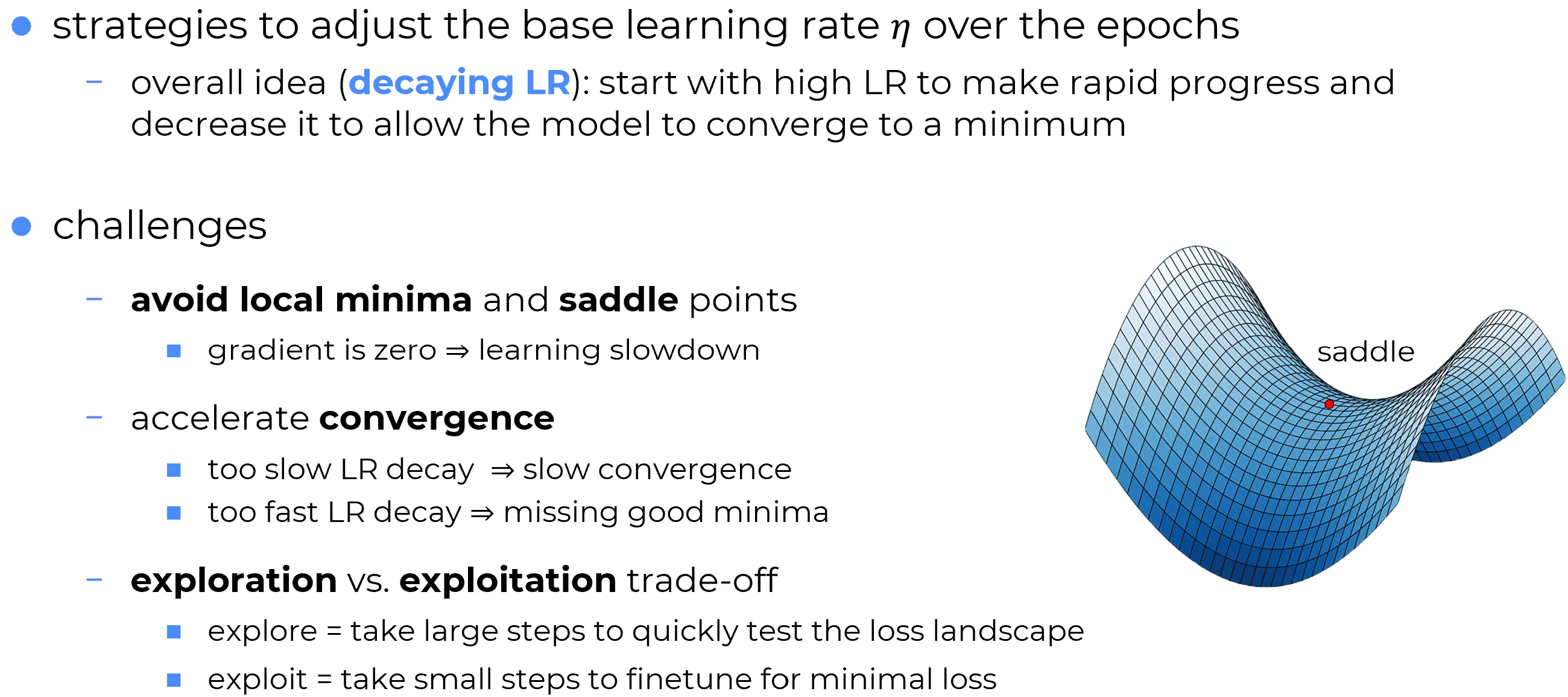
In high-dimensional nonconvex optimization, the most common slow-down is not a “bad local minimum” but a saddle-like neighbourhood in which the gradient nearly vanishes along most directions while remaining non-zero along a few. A learning rate that is too small lets the optimizer drift through such regions; a learning rate that is large enough preserves enough kinetic effect to leave them efficiently. The choice of the early-training learning rate is therefore not just about speed: it can determine whether the optimizer escapes saddle regions at all within the training budget.

3. What a scheduler actually controls

A scheduler defines a function

$${\eta }_t:\text{(scheduler step)}\to \text{(learning rate)},$$

evaluated at every call to scheduler.step().

Scheduler steps are not intrinsically epochs

The unit of time used by the scheduler is not intrinsically an epoch. It is whatever scheduler.step() is called against:

• if step() is called once per epoch, scheduler time counts epochs;
• if step() is called once per iteration, scheduler time counts iterations.

The hyperparameters of every scheduler (step_size, T_max, T_0, gamma, …) must be expressed in the same time unit as the stepping frequency. Mixing the two (e.g.\ stepping per batch while picking T_max in epochs) is the most common cause of “the scheduler did nothing” or “the scheduler decayed to zero in the first epoch” bugs. The detailed implications for individual schedulers are in Step and Exponential decay and Cosine annealing.

A scheduler is therefore defined by three ingredients, not just by its formula:

1. the formula ${\eta }_t$ (step, exponential, cosine, …);
2. the stepping frequency at which scheduler.step() is called;
3. the time horizon over which the schedule is meant to play out.

A schedule “works” only when all three are consistent with each other.

4. The three ingredients of a scheduling pipeline

Most real-world scheduling pipelines are compositions of at most three orthogonal components, each addressing a different phase of training.

component	phase of training	role
warm-up	startup	ramp the learning rate up from a small value to ${\eta }_{\max }$, stabilizing the first few hundred or few thousand iterations
main decay	bulk descent	reduce $\eta$ from ${\eta }_{\max }$ to ${\eta }_{\min }$ over the main training horizon; choice between exponential and cosine decay
restarts	late descent / multi-cycle	optionally repeat the main decay multiple times, allowing renewed exploration phases and snapshot ensembles

These components are not redundant

A common mistake is to add scheduler complexity without distinguishing what each component is for. Each of the three ingredients above addresses a different failure mode:

• warm-up addresses startup instability (especially for Adam / AdamW, whose moment estimates are noisy in the first iterations);
• monotone decay addresses the exploration-to-exploitation transition during the main descent;
• restarts address the limitation of a single decay trajectory ending in a possibly-mediocre basin.

Replacing any of the three with another does not solve the same problem. A scheduling pipeline that combines all three (e.g.\ linear warm-up + cosine decay + SGDR-style restarts) is doing something substantively different from one that uses only a single component, and the components should be chosen with their distinct roles in mind.

The decision of which combination to use, and how to set the relevant hyperparameters, is the subject of Choosing an LR scheduler. The mechanics of each individual family are in the next two notes.

5. Where to read about each family

The two foundational families and one modern default are treated in dedicated notes:

• Step Decay: piecewise-constant schedule that drops $\eta$ by a factor $\gamma$ every fixed interval. Explicit milestone-based regime changes.
• Exponential Decay: smooth monotone decay ${\eta }_n={\eta }_0{\gamma }^n$. Continuous contraction at every step, single tuning knob.
• Cosine Annealing: smooth half-cosine from ${\eta }_{\max }$ to ${\eta }_{\min }$, optionally with warm restarts. The de-facto default for modern Transformer-scale training when paired with linear warm-up.

These are more than different formulas: they represent different answers to the broader question of how training dynamics should evolve over time.

6. Summary

Final takeaway

Adaptive optimizers determine how learning rates differ across parameters. Learning-rate schedulers determine how the base learning rate evolves over time. A complete optimization pipeline often needs both, and a strong scheduler is one whose formula, stepping frequency, and time horizon are consistent with each other.

Practical scheduler design is the subject of Choosing an LR scheduler; the mechanics of the individual families are developed in Step and Exponential decay and Cosine annealing.