Nesterov momentum

Why this method is historically important

Nesterov momentum matters for two distinct reasons:

• practical dynamics: improved trajectory control compared with classical momentum;
• theory: accelerated convergence in smooth convex optimization.

For smooth convex objectives:

• gradient descent has rate $\mathcal{O}(1/k)$;
• Nesterov acceleration reaches $\mathcal{O}(1/k^2)$.

This rate improvement is the historical core of Nesterov’s contribution.

Convex-function assumptions used below (notation-aligned)

The classical assumptions are:

• Convexity: $$f(y)\ge f(x)+\nabla f(x{)}^{\top }(y-x).$$
• $\alpha$-strong convexity, when needed: $$f(y)\ge f(x)+\nabla f(x{)}^{\top }(y-x)+\frac{\alpha }{2}\Vert y-x{\Vert }^2.$$
• $L$-smoothness / Lipschitz gradient: $$f(y)\le f(x)+\nabla f(x{)}^{\top }(y-x)+\frac{L}{2}\Vert y-x{\Vert }^2.$$

Why $\mathcal{O}(1/k)$ for GD and $\mathcal{O}(1/k^2)$ for Nesterov? (compact sketch)

Consider convex and $L$-smooth $f$, with gradient descent:

$${\mathbf{\theta }}^{(k+1)}={\mathbf{\theta }}^{(k)}-\frac{1}{L}\nabla f\left({\mathbf{\theta }}^{(k)}\right).$$

By smoothness:

$$f\left({\mathbf{\theta }}^{(k+1)}\right)\le f\left({\mathbf{\theta }}^{(k)}\right)-\frac{1}{2L}{\Vert \nabla f\left({\mathbf{\theta }}^{(k)}\right)\Vert }^2.$$

By convexity at ${\mathbf{\theta }}^{\star }\in \arg \min f$:

$$f\left({\mathbf{\theta }}^{(k)}\right)-f({\mathbf{\theta }}^{\star })\le \nabla f{\left({\mathbf{\theta }}^{(k)}\right)}^{\top }\left({\mathbf{\theta }}^{(k)}-{\mathbf{\theta }}^{\star }\right).$$

Expanding the distance recursion:

$${\Vert {\mathbf{\theta }}^{(k+1)}-{\mathbf{\theta }}^{\star }\Vert }^2={\Vert {\mathbf{\theta }}^{(k)}-{\mathbf{\theta }}^{\star }\Vert }^2-\frac{2}{L}\nabla f{\left({\mathbf{\theta }}^{(k)}\right)}^{\top }\left({\mathbf{\theta }}^{(k)}-{\mathbf{\theta }}^{\star }\right)+\frac{1}{L^2}{\Vert \nabla f\left({\mathbf{\theta }}^{(k)}\right)\Vert }^2.$$

Combining and telescoping gives:

$$f\left({\mathbf{\theta }}^{(k)}\right)-f({\mathbf{\theta }}^{\star })\le \frac{L{\Vert {\mathbf{\theta }}^{(0)}-{\mathbf{\theta }}^{\star }\Vert }^2}{2k},$$

hence $\mathcal{O}(1/k)$.

For Nesterov acceleration, estimate-sequence / potential arguments yield:

$$f(y_k)-f({\mathbf{\theta }}^{\star })\le \mathcal{O}\left(\frac{L{\Vert {\mathbf{\theta }}^{(0)}-{\mathbf{\theta }}^{\star }\Vert }^2}{k^2}\right),$$

hence $\mathcal{O}(1/k^2)$.

Scope of the rate claim

The $\mathcal{O}(1/k^2)$ statement belongs to deterministic smooth convex optimization. Deep-learning training is usually stochastic and nonconvex, so this theorem is not transferred directly.

---

2. NAG equations

Notation:

• ${\mathbf{\theta }}^{(t)}$: parameters at iteration $t$;
• ${\mathbf{v}}^{(t)}$: velocity/update vector;
• $\eta >0$: learning rate;
• $\mu \in [0,1)$: momentum coefficient.

What inertia means in momentum methods

Inertia is persistence of update direction across iterations. In

$${\mathbf{v}}^{(t)}=\mu {\mathbf{v}}^{(t-1)}-\eta {\mathbf{g}}^{(t)},$$

the term $\mu {\mathbf{v}}^{(t-1)}$ carries part of the previous update into the current step.

Unrolling the recurrence:

$${\mathbf{v}}^{(t)}={\mu }^t{\mathbf{v}}^{(0)}-\eta \sum _{j=0}^{t-1}{\mu }^j{\mathbf{g}}^{(t-j)}.$$

With ${\mathbf{v}}^{(0)}=0$, velocity is an exponentially weighted accumulation of recent gradients.

• larger $\mu$: longer memory and stronger inertial carry-over;
• smaller $\mu$: shorter memory and more reactive updates.

NAG keeps the same inertial mechanism; the difference is where the gradient is evaluated (look-ahead point instead of current point).

Component	Classical momentum	Nesterov momentum
Velocity update	${\mathbf{v}}^{(t)}=\mu {\mathbf{v}}^{(t-1)}-\eta {\nabla }_{\mathbf{\theta }}\mathcal{L}\left({\mathbf{\theta }}^{(t)}\right)$	${\mathbf{v}}^{(t)}=\mu {\mathbf{v}}^{(t-1)}-\eta {\nabla }_{\mathbf{\theta }}\mathcal{L}\left({\mathbf{\theta }}^{(t)}+\mu {\mathbf{v}}^{(t-1)}\right)$
Parameter update	${\mathbf{\theta }}^{(t+1)}={\mathbf{\theta }}^{(t)}+{\mathbf{v}}^{(t)}$	${\mathbf{\theta }}^{(t+1)}={\mathbf{\theta }}^{(t)}+{\mathbf{v}}^{(t)}$
Gradient evaluation point	${\mathbf{\theta }}^{(t)}$	${\mathbf{\theta }}^{(t)}+\mu {\mathbf{v}}^{(t-1)}$
Intuition	reactive correction at current location	anticipatory correction at look-ahead location

Equivalent predictor-corrector form

Define

$${\tilde{\mathbf{\theta }}}^{(t)}\triangleq {\mathbf{\theta }}^{(t)}+\mu {\mathbf{v}}^{(t-1)}.$$

Then NAG can be written as:

$${\mathbf{v}}^{(t)}={\tilde{\mathbf{\theta }}}^{(t)}-{\mathbf{\theta }}^{(t)}-\eta {\nabla }_{\mathbf{\theta }}\mathcal{L}\left({\tilde{\mathbf{\theta }}}^{(t)}\right),$$

which makes the predict-then-correct mechanism explicit.

Concise intuition: classical momentum reacts after displacement, while Nesterov momentum evaluates the slope at the anticipated position and corrects during displacement formation.

Why this can help even in nonconvex stochastic training

Strict convex acceleration guarantees may not apply. Nevertheless, earlier directional correction often improves practical stability:

• less delay between inertial drift and gradient feedback;
• better damping in stiff directions;
• cleaner behavior under aggressive learning-rate schedules.

---

3. Geometric refinement over classical momentum

A full explanation of Nesterov look-ahead behavior requires moving beyond the gradient $\nabla \mathcal{L}$ and considering local curvature through the Hessian matrix $\mathbf{H}$.

General loss-landscape geometry, including saddle points, is discussed in gradient descent.
The ravine geometry in which inertia becomes especially useful is developed in momentum.

The present note isolates what is specific to Nesterov momentum. Once the optimization trajectory is already understood as moving through an anisotropic valley, NAG modifies the dynamics by evaluating the gradient at a look-ahead point rather than at the current parameters.

This means that curvature influences the correction earlier in the step construction. The practical effect is often a shorter cross-valley excursion and a more anticipatory damping of inertial overshoot than in classical momentum.

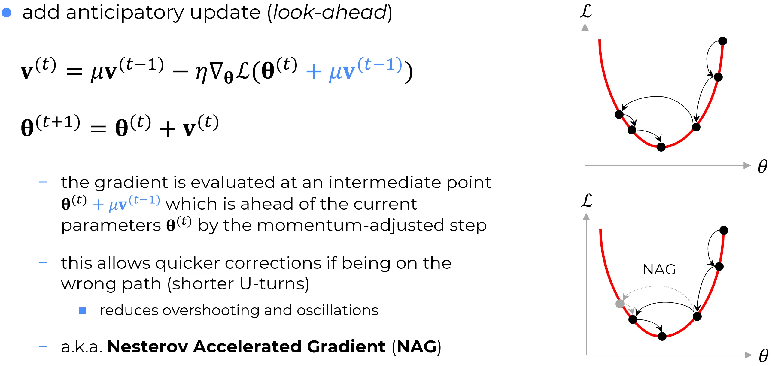
How to read the figure

The upper panel illustrates a longer oscillatory trajectory associated with classical momentum. The lower panel illustrates NAG: the gray look-ahead marker indicates where the corrective gradient is queried before the update is finalized. The visual message is geometric and dynamical, not merely algebraic notation.

---

4. 1D quadratic case: NAG damping made explicit

Section objective

The goal of this section is to isolate the NAG mechanism in the simplest setting where every step is explicit:

• show exactly where curvature enters the momentum channel;
• explain why steep curvature requires stronger damping;
• prepare the multidimensional interpretation, where each Hessian eigendirection behaves like this same scalar mode with $a={\lambda }_i$.

Consider the one-dimensional quadratic model

$$\mathcal{L}(\theta )=\frac{a}{2}{\theta }^2,a>0.$$

Then $\nabla \mathcal{L}(\theta )=a\theta$, so NAG gives

$$v^{(t)}=\mu v^{(t-1)}-\eta a({\theta }^{(t)}+\mu v^{(t-1)})=\mu (1-\eta a)v^{(t-1)}-\eta a{\theta }^{(t)}.$$

Classical momentum is

$$v^{(t)}=\mu v^{(t-1)}-\eta a{\theta }^{(t)}.$$

So the structural difference is exact:

• classical momentum carries inertia with factor $\mu$;
• NAG carries inertia with factor $\mu (1-\eta a)$.

Interpretation

• the inherited-velocity contribution is exactly the term $\mu (1-\eta a)v^{(t-1)}$;
• if $a$ is small, then $(1-\eta a)\approx 1$, so the multiplier stays close to $\mu$ and more of the previous velocity is preserved (more inertial memory);
• if $a$ is large, then $|1-\eta a|$ moves away from $1$ and inherited velocity is attenuated more strongly (and may even flip sign when $\eta a>1$).

Including the parameter update ${\theta }^{(t+1)}={\theta }^{(t)}+v^{(t)}$, the linear homogeneous dynamics can be written as

$$\left[\begin{array}{c}{\theta }^{(t+1)}\\ v^{(t)}\end{array}\right]=\left[\begin{array}{cc}1-\eta a& \mu (1-\eta a)\\ -\eta a& \mu (1-\eta a)\end{array}\right]\left[\begin{array}{c}{\theta }^{(t)}\\ v^{(t-1)}\end{array}\right].$$

How to read the stability condition

This is a linear time-discrete dynamical system of the form $x_t=\mathbf{A}{x}_{t-1}$ with

$$x_t=\left[\begin{array}{c}{\theta }^{(t+1)}\\ v^{(t)}\end{array}\right],\mathbf{A}=\left[\begin{array}{cc}1-\eta a& \mu (1-\eta a)\\ -\eta a& \mu (1-\eta a)\end{array}\right].$$

Local asymptotic stability means that trajectories converge to zero, which for linear discrete systems is equivalent to all eigenvalues of $\mathbf{A}$ lying inside the unit disk:

$$|{\lambda }_i(\mathbf{A})|<1⟺\rho (\mathbf{A})<1.$$

Here $\rho (\mathbf{A})$ is the spectral radius, i.e. $\rho (\mathbf{A})={\max }_i|{\lambda }_i(\mathbf{A})|$. The scalar inequality $|\mu (1-\eta a)|<1$ checks only the coefficient multiplying $v^{(t-1)}$ in the $v^{(t)}$ update, so it is an intuition cue, not a full stability test. Practical takeaway: when curvature $a$ increases, stable learning-rate range typically shrinks.

---

5. Extended Hessian analysis

The multidimensional picture is the exact extension of the 1D template above: each Hessian eigendirection behaves like a scalar mode with $a={\lambda }_i$.

Assume $\mathcal{L}$ is twice differentiable near ${\mathbf{\theta }}^{(t)}$, with local Hessian ${\mathbf{H}}_t$. Taylor expansion around ${\mathbf{\theta }}^{(t)}$ gives:

$$\nabla \mathcal{L}\left({\mathbf{\theta }}^{(t)}+\mu {\mathbf{v}}^{(t-1)}\right)\approx \nabla \mathcal{L}\left({\mathbf{\theta }}^{(t)}\right)+{\mathbf{H}}_t\left(\mu {\mathbf{v}}^{(t-1)}\right).$$

Why ${\mathbf{H}}_t$ is symmetric, and why eigenvalues are real

For $\mathcal{L}\in {\mathcal{C}}^2$, mixed second derivatives are continuous. By Schwarz-Clairaut:

$$\frac{{\partial }^2\mathcal{L}}{\partial {\theta }_i\partial {\theta }_j}=\frac{{\partial }^2\mathcal{L}}{\partial {\theta }_j\partial {\theta }_i},$$

hence $({\mathbf{H}}_t{)}_{ij}=({\mathbf{H}}_t{)}_{ji}$, so ${\mathbf{H}}_t$ is real symmetric. A real symmetric matrix has:

• real eigenvalues;
• an orthonormal eigenbasis.

This is exactly the hypothesis of the spectral theorem used below.

Taylor remainder (what is hidden by $\approx$)

The first-order expansion of the gradient is

$$\nabla \mathcal{L}(\theta +\Delta )=\nabla \mathcal{L}(\theta )+\mathbf{H}(\theta )\Delta +\mathbf{r}(\Delta ),\Vert \mathbf{r}(\Delta )\Vert =\mathcal{O}(\Vert \Delta {\Vert }^2).$$

Here $\Delta =\mu {\mathbf{v}}^{(t-1)}$. So the approximation is accurate when the look-ahead displacement is locally small and Hessian variation over that displacement is limited.

Substituting into NAG:

$${\mathbf{v}}^{(t)}\approx \mu {\mathbf{v}}^{(t-1)}-\eta \nabla \mathcal{L}\left({\mathbf{\theta }}^{(t)}\right)-\eta \mu {\mathbf{H}}_t{\mathbf{v}}^{(t-1)}.$$

Therefore:

$${\mathbf{v}}^{(t)}\approx \mu (\mathbf{I}-\eta {\mathbf{H}}_t){\mathbf{v}}^{(t-1)}-\eta \nabla \mathcal{L}\left({\mathbf{\theta }}^{(t)}\right).$$

The extra curvature-dependent term is:

$$-\eta \mu {\mathbf{H}}_t{\mathbf{v}}^{(t-1)}.$$

It modulates inherited inertia before the update is finalized. This is the formal mechanism behind look-ahead damping.

Deep dive: eigen-direction decomposition (and why it is valid)

The decomposition

$${\mathbf{H}}_t=\mathbf{Q\Lambda }{\mathbf{Q}}^{\top }$$

is not an arbitrary assumption. By the spectral theorem, every real symmetric matrix is orthogonally diagonalizable:

• $\mathbf{Q}=[{\mathbf{q}}_1,\dots ,{\mathbf{q}}_d]$ has orthonormal eigenvectors;
• $\mathbf{\Lambda }=\mathrm{diag}({\lambda }_1,\dots ,{\lambda }_d)$ contains real eigenvalues.

Minimal proof sketch for real eigenvalues: if $\mathbf{Hu}=\lambda \mathbf{u}$ with $\mathbf{u}\ne 0$, then

$$\lambda =\frac{{\mathbf{u}}^{\top }\mathbf{Hu}}{{\mathbf{u}}^{\top }\mathbf{u}},$$

and the right-hand side is real because $\mathbf{H}$ is real symmetric.

Any vector admits expansion on this orthonormal basis:

$${\mathbf{v}}^{(t-1)}=\sum _i{\alpha }_i{\mathbf{q}}_i,{\alpha }_i={\mathbf{q}}_i^{\top }{\mathbf{v}}^{(t-1)}.$$

Applying the NAG attenuation operator:

$$\begin{array}{rl}(\mathbf{I}-\eta {\mathbf{H}}_t){\mathbf{v}}^{(t-1)}& =(\mathbf{I}-\eta {\mathbf{H}}_t)\sum _i{\alpha }_i{\mathbf{q}}_i\\ & =\sum _i{\alpha }_i(\mathbf{I}-\eta {\mathbf{H}}_t){\mathbf{q}}_i\\ & =\sum _i{\alpha }_i(1-\eta {\lambda }_i){\mathbf{q}}_i.\end{array}$$

Hence:

$$(\mathbf{I}-\eta {\mathbf{H}}_t){\mathbf{v}}^{(t-1)}=\sum _i(1-\eta {\lambda }_i){\alpha }_i{\mathbf{q}}_i.$$

Interpretation of each factor:

• ${\alpha }_i$: inherited velocity component in eigendirection ${\mathbf{q}}_i$;
• $(1-\eta {\lambda }_i)$: direction-specific gain set by local curvature.

Components aligned with large positive ${\lambda }_i$ (steep directions) are attenuated more strongly. This is the linear-algebraic origin of steep-direction damping.

Intuition after the algebra

Each eigendirection behaves like an independent one-dimensional mode. The factor $(1-\eta {\lambda }_i)$ acts as a mode-specific brake:

• steep mode (${\lambda }_i$ large): aggressive braking;
• flat mode (${\lambda }_i$ small): mild braking.

NAG therefore reshapes inertia by geometry, not by a single global scalar.

Deep dive: hardware reality (why ${\mathbf{H}}^{-1}$ is usually infeasible)

Newton’s method would use

$${\mathbf{\theta }}^{(t+1)}={\mathbf{\theta }}^{(t)}-{\mathbf{H}}^{-1}\nabla \mathcal{L}.$$

For a model with about $25.6$ million parameters (ResNet-50 scale), the dense Hessian size is

$$n^2\approx 6.55\times 10^{14}\text{ entries}.$$

In float32, storage alone is about

$$4n^2\approx 2.62\times 10^{15}\text{ bytes}\approx 2.6\text{ PB}.$$

Direct inversion scales as $\mathcal{O}(n^3)$, which is computationally prohibitive per training step. This is why deep learning relies on first-order optimizers. NAG is an engineering compromise: first-order cost with implicit second-order curvature behavior.

---

6. Conceptual look-ahead vs PyTorch implementation

The canonical NAG equation explicitly uses

$$\nabla \mathcal{L}\left({\mathbf{\theta }}^{(t)}+\mu {\mathbf{v}}^{(t-1)}\right).$$

torch.optim.SGD implements Nesterov through a momentum-buffer state computed from current-parameter gradients:

• $g_t=\nabla f_t({\theta }_{t-1})$ (plus optional weight decay);
• buffer update $$b_t=\{\begin{array}{ll}{g}_t,& t=1,\\ \mu b_{t-1}+(1-\tau )g_t,& t>1;\end{array}$$
• Nesterov direction: $d_t=g_t+\mu b_t$;
• parameter step: ${\theta }_t={\theta }_{t-1}-\gamma d_t$.

What the buffer actually stores

The buffer $b_t$ stores gradient history, not parameter history. With $\tau =0$:

$$b_t=\mu b_{t-1}+g_t.$$

Expanding the first steps:

$$b_1=g_1,b_2=\mu g_1+g_2,b_3={\mu }^2{g}_1+\mu g_2+g_3.$$

So each new buffer is a weighted sum of recent gradients, with geometric decay by powers of $\mu$. This weighted accumulation is exactly what “momentum memory” means.

Where PyTorch computes the gradient in Nesterov mode

Canonical NAG writes

$$\nabla \mathcal{L}\left({\theta }_{t-1}+\mu v_{t-1}\right),$$

i.e. gradient at a shifted point. PyTorch does not run an explicit second forward/backward at that shifted point. It computes one gradient at current parameters,

$$g_t=\nabla \mathcal{L}({\theta }_{t-1}),$$

then builds the Nesterov direction algebraically:

$$d_t=g_t+\mu b_t,{\theta }_t={\theta }_{t-1}-\gamma d_t.$$

So the look-ahead effect is implemented through direction construction, not through an explicit extra gradient query.

---

7. Sutskever’s step notation and its relation to PyTorch

Historical note

A very influential deep-learning presentation of momentum is the one used in Sutskever, Martens, Dahl, and Hinton (2013), On the importance of initialization and momentum in deep learning. In that notation, the state variable is the parameter step itself, not an unscaled momentum buffer.

Since many references still use the Sutskever convention, without making that convention explicit, PyTorch formulas can look different even when they describe the same underlying dynamics.

Sutskever-style notation writes the state as the step applied to the parameters:

$$s_{t+1}=\mu s_t+\text{lr}{g}_{t+1},p_{t+1}=p_t-s_{t+1}.$$

Interpretation:

• $s_t$ already includes learning-rate scaling;
• the parameter update is simply “subtract the step.”

PyTorch-style notation instead stores an unscaled momentum buffer:

$$m_{t+1}=\mu m_t+g_{t+1},p_{t+1}=p_t-\text{lr}{m}_{t+1}.$$

Here $m_t$ is the same object denoted by $b_t$ in Section 6.

The real difference

The two formulas do not introduce two different optimizers. They define the internal state differently:

• Sutskever: state = already-scaled step;
• PyTorch: state = unscaled gradient accumulator.

If learning rate is constant, the mapping is immediate.

Define

$$s_t\triangleq \text{lr}{m}_t.$$

Then

$$s_{t+1}=\text{lr}{m}_{t+1}=\text{lr}(\mu m_t+g_{t+1})=\mu s_t+\text{lr}{g}_{t+1},$$

and

$$p_{t+1}=p_t-\text{lr}{m}_{t+1}=p_t-s_{t+1}.$$

So under constant learning rate, the Sutskever formula is just the PyTorch formula written in a different state variable.

Why schedules break the exact equivalence

If learning rate changes over time, define $s_t={\text{lr}}_t{m}_t$. Then

$$s_{t+1}=\mu \frac{{\text{lr}}_{t+1}}{{\text{lr}}_t}{s}_t+{\text{lr}}_{t+1}{g}_{t+1}.$$

The extra ratio ${\text{lr}}_{t+1}/{\text{lr}}_t$ means the momentum memory is rescaled when the schedule changes. This is why the two conventions can have different transient behavior under learning-rate schedules even if they coincide when learning rate is constant.

Nesterov variants follow the same logic.

Summary

The important point is not “which formula is correct,” but “what quantity the state variable is supposed to represent.”

---

8. Practical PyTorch recipe

import torch
 
optimizer = torch.optim.SGD(
    model.parameters(),
    lr=0.1,
    momentum=0.9,
    nesterov=True,
    weight_decay=1e-4,
    dampening=0.0,
)

Note

In PyTorch, nesterov=True requires momentum > 0 and dampening = 0.

---

9. Final summary

Nesterov momentum is most robustly understood through three coordinated layers:

1. conceptual: look-ahead gradient correction;
2. geometric: curvature-shaped damping through $(\mathbf{I}-\eta {\mathbf{H}}_t)$;
3. engineering: efficient first-order implementation used in modern frameworks.

This explains why NAG remains relevant: it preserves first-order scalability while embedding useful curvature-aware behavior.

---

10. Primary references

• Yurii Nesterov, A method for solving the convex programming problem with convergence rate $O(1/k^2)$ (1983)
• Ilya Sutskever, James Martens, George Dahl, Geoffrey Hinton, On the importance of initialization and momentum in deep learning
• PyTorch documentation, torch.optim.SGD: https://pytorch.org/docs/stable/generated/torch.optim.SGD.html
• Ian Goodfellow, Yoshua Bengio, Aaron Courville, Deep Learning