Overfitting on MNIST

Experiment 1 – Reduced Dataset

Architecture setup

Let’s consider a simple MLP composed of:

an input layer with $784$ neurons (i.e., one for each pixel of the $28 \times 28$ flattened MNIST images)

a single hidden layer with $30$ neurons

an output layer with $10$ neurons corresponding to the digit classes.

In total, this network has $23, 860$ parameters.

Parameter count of the MLP

Input → Hidden (784 × 30): 23,520 weights + 30 biases = 23,550

Hidden → Output (30 × 10): 300 weights + 10 biases = 310

Total = 23,860 parameters

Note

Suppose the network is trained not on the full set of $50, 000$ MNIST training images, but only on the first $1, 000$ .
This restriction makes the problem of generalization even more evident.

Training setup

The training setup includes:

the use of Cross-Entropy as the loss function,

a learning rate of $η = 0.5$ ,

a mini-batch size of $10$ ,

a total of $400$ epochs — a higher-than-usual value, chosen to compensate for the reduced number of training samples.

Results

Training Loss and Test Accuracy

Training Loss	Test Accuracy

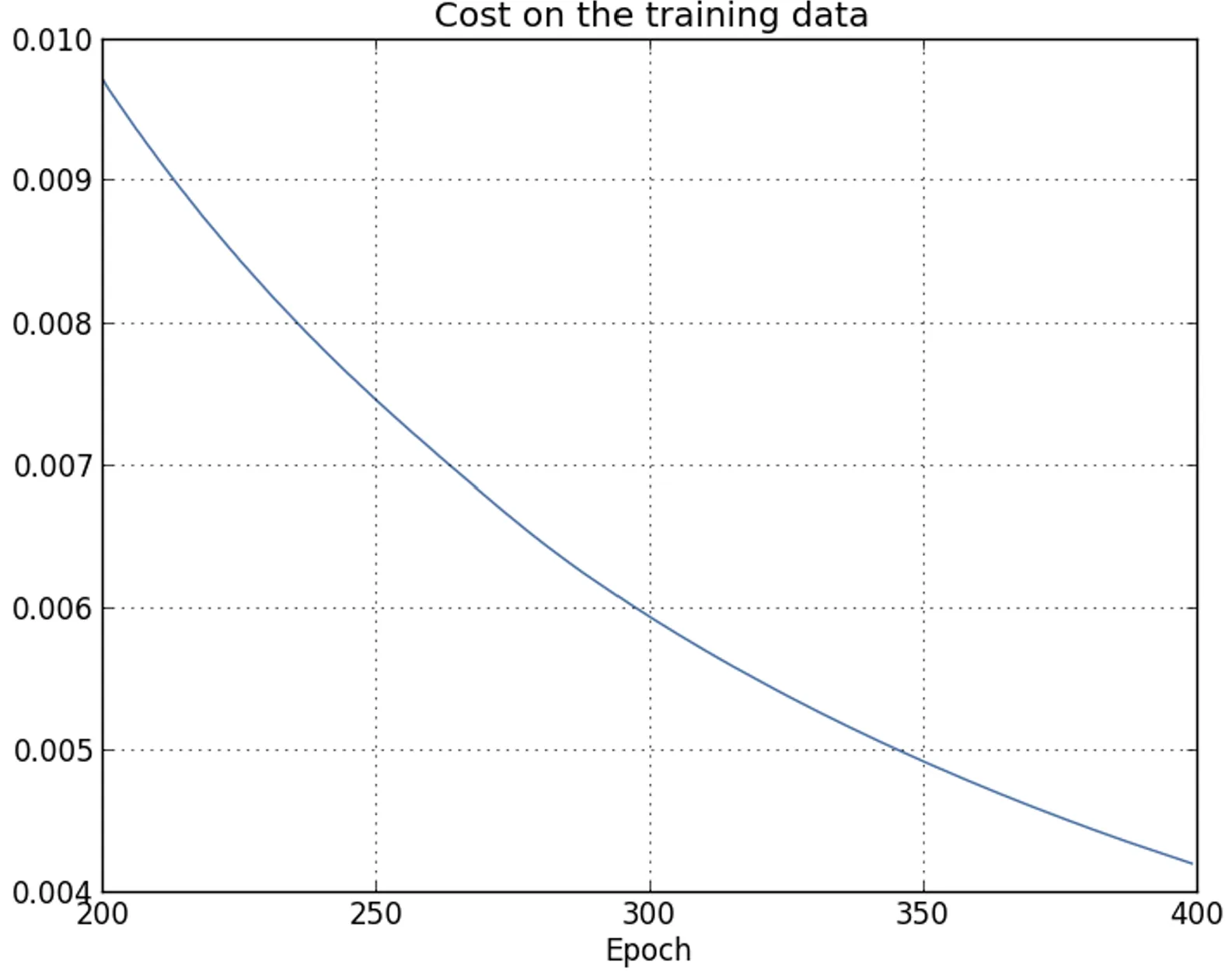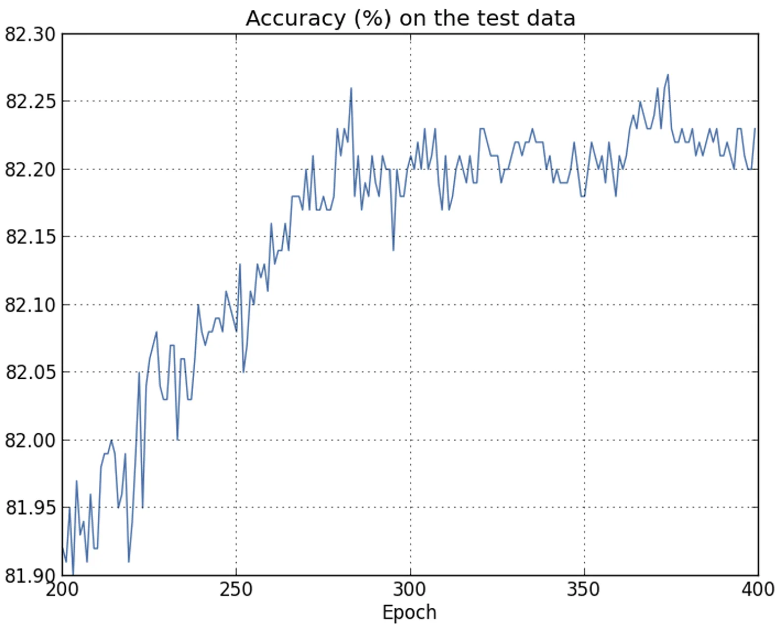The result appears promising, with a steady decrease in the loss as expected. Only the training epochs from $200$ to $399$ are shown, providing a zoomed-in view of the final phases of learning, which turn out to be particularly insightful.	Here as well, the plot shows a magnified detail. In the first $200$ epochs (not shown), accuracy increases to just under $82%$ . Subsequently, learning gradually slows down. Around epoch $280$ , classification accuracy stabilizes, with no further significant improvements. The following epochs display only slight stochastic fluctuations around the value reached at that point.

Important

Unlike what is suggested by the training loss curve, which continues to decrease steadily, the test accuracy results show that this apparent improvement is actually an illusion.

As in the model criticized by Fermi, what the network learns after epoch $280$ no longer generalizes to unseen data and therefore does not constitute useful learning.
At this stage, the phenomenon is referred to as overfitting or overtraining.

Question

One might wonder whether the issue lies in comparing the training loss with the test classification accuracy. In other words:

Could the problem stem from contrasting heterogeneous metrics?

What would happen by comparing the training with the test loss or classification accuracy on both the training and test data, thus enabling a comparison between homogeneous metrics?

In fact, the same fundamental phenomenon emerges regardless of the chosen comparison methodology.
However, certain specific aspects do vary.

Training and Test Loss

As an illustrative example, consider the loss computed on the test data:

Training loss	Loss on Test Data

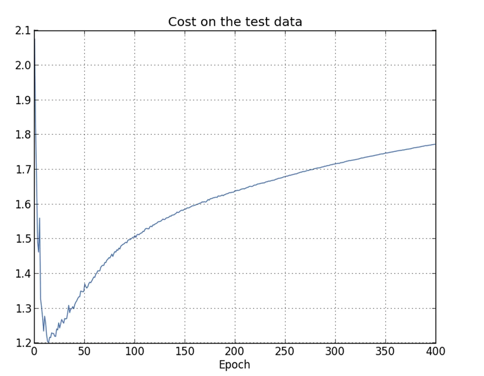It can be observed that the test loss improves until about epoch $15$ , but beyond that point it actually starts to worsen, even though the training loss continues to decrease.

This provides further evidence that the model is experiencing overfitting. However, it also raises a key question:

Question

Should epoch $15$ or epoch $280$ be considered the point at which overfitting begins to dominate the learning process?

Answer

From a practical standpoint, the primary goal is to improve classification accuracy on the test data, while the loss on such data serves only as a surrogate for that accuracy.
This is because the loss (e.g., cross-entropy) provides a continuous and differentiable proxy that guides optimization, whereas accuracy is a discrete metric that directly measures prediction correctness.
As a result, it is more reasonable to identify epoch $280$ as the point beyond which overfitting dominates the learning process in the neural network.

Training and Test Accuracy

An additional indicator of overfitting can be observed in the classification accuracy on the training data:

Training Accuracy	Test Accuracy

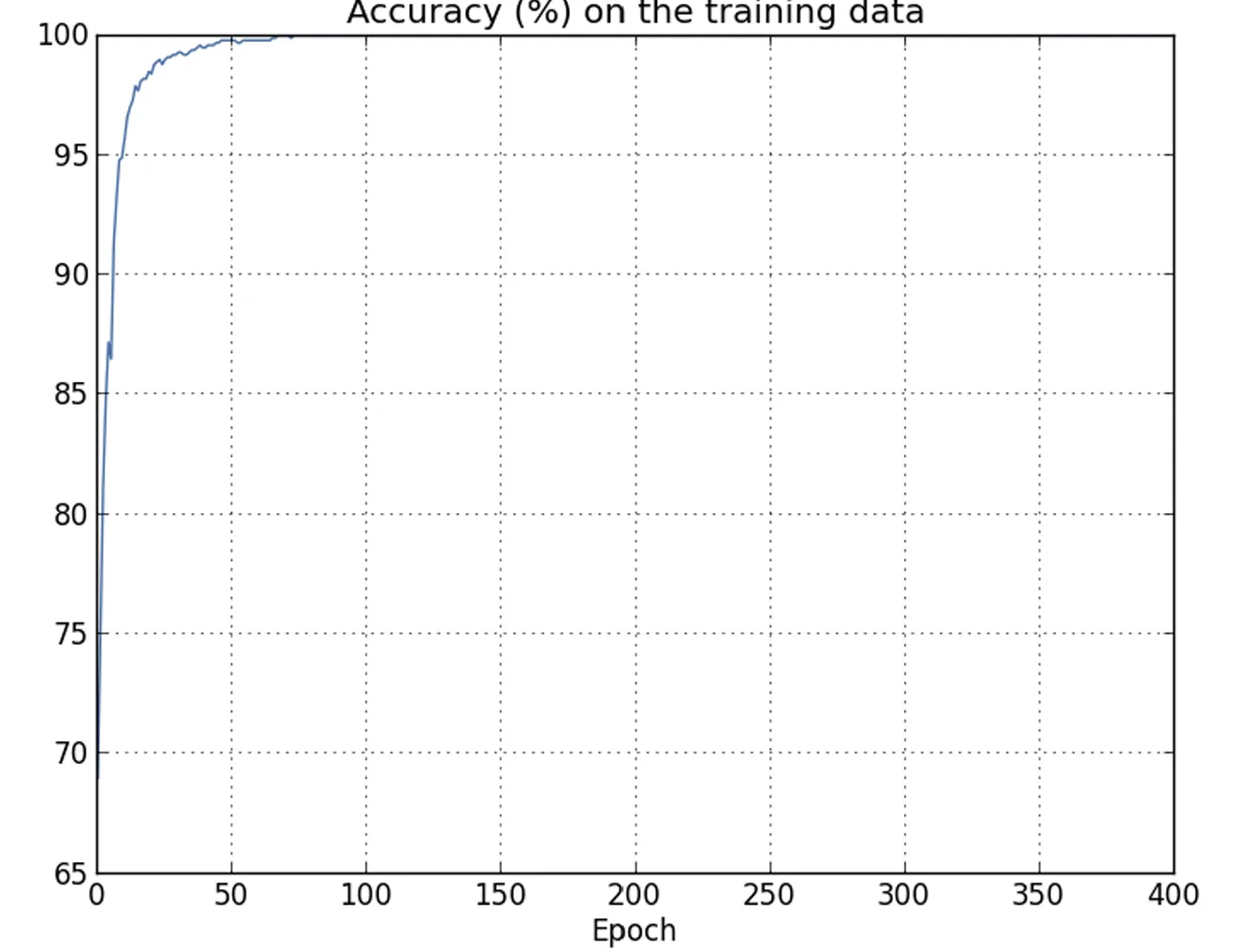Training accuracy progressively reaches 100%. In other words, the network correctly classifies all $1, 000$ training images.	By contrast, test accuracy stabilizes at a maximum of 82.27%.

Note

This shows that the network is learning peculiarities specific to the training set rather than recognizing digits in a generalized way.
It is as if the network were merely memorizing the training set without developing a sufficient understanding of the digits to generalize to the test data.

Important

Overfitting represents a critical issue in neural networks, particularly in modern architectures that often contain an extremely large number of weights and biases.
For effective training, it is essential to identify when overfitting occurs, thereby avoiding overtraining.
In addition, it is also necessary to employ techniques to mitigate the effects of overfitting.

Overfitting mitigation

Early Stopping (with Test Set)

Basic Strategy

The most straightforward method to detect overfitting is to monitor test accuracy during training, as illustrated earlier.
If it is observed that test accuracy no longer improves, training should be stopped.

Note

However, it is important to note that such stagnation does not necessarily represent an unequivocal signal of overfitting. It may in fact occur that both test and training accuracy stop improving simultaneously. Nevertheless, adopting this strategy effectively prevents overfitting.

In what follows, a variant of this strategy will be employed.

Using a Validation set

Note

So far, only the training_data and the test_data have been used, while the validation_data has been ignored.

Info

The validation_data consists of $10, 000$ digit images, distinct from the $50, 000$ images in the MNIST training set and the $10, 000$ images in the test set.

Early stopping (with Validation Set)

Instead of using the test_data to prevent overfitting, the validation_data will be employed.
To this end, a strategy similar to the one previously described for the test_data will be adopted: the classification accuracy on the validation_data will be computed at the end of each epoch.
Once the accuracy on the validation_data stabilizes, training is stopped.
This strategy is known as early stopping.

Note

Of course, in practice it is not possible to determine immediately the exact point at which accuracy saturates. Training is therefore continued until there is sufficient evidence that accuracy has reached a plateau.

Question

Why use validation_data instead of test_data to address overfitting?

Answer

This choice is part of a broader strategy, which involves using validation_data to evaluate different hyperparameter configurations, such as the number of epochs, the learning rate, the network architecture, and so on.
Such evaluations make it possible to identify optimal values for the hyperparameters.

However, this does not explain why validation_data is preferred over test_data to prevent overfitting.
The key issue lies in why validation_data is prioritized over test_data during hyperparameter tuning.

Important

To understand this, note that the search for optimal hyperparameters involves exploring a wide hyperparameter search space through multiple experimental configurations.
If these choices were based on the test_data, there would be a risk of overfitting the hyperparameters to the test set, capturing its specific peculiarities rather than ensuring effective generalization.

Hold-out method

To avoid this, hyperparameters are optimized on the validation_data. Only afterwards is the final performance evaluated on the test_data, providing a reliable measure of the network’s generalization ability.
In other words, the validation_data acts as a “training set for hyperparameters.”
This methodology is known as the hold-out method, since the validation_data is kept separate (or “held out”) from the training_data.

The Risk of Test Set Overfitting

In practice, even after evaluating the model on the test_data, one might decide to modify the approach (for example, by adopting a different network architecture), which would imply a new round of hyperparameter optimization.
This raises the concern of potential overfitting on the test_data, theoretically requiring an infinite series of datasets to fully guarantee generalization.
Although this is a complex issue, in practical scenarios the basic hold-out method is applied, based on the tripartition training_data / validation_data / test_data.

After analyzing overfitting with the reduced dataset, the phenomenon can now be examined in the context of the full dataset.

Experiment 2 – Full Dataset

Up to now, overfitting has been analyzed using $1, 000$ training images.

Question

What happens when the entire training set of $50, 000$ images is used?

Experiment Setup

Keeping the other parameters unchanged ( $30$ hidden neurons, learning rate $0.5$ , mini-batch size $10$ ), training is performed for $30$ epochs.

Results

The following plot shows the classification accuracy on both the training data and the test data (the latter included here for consistency with the previous comparisons).

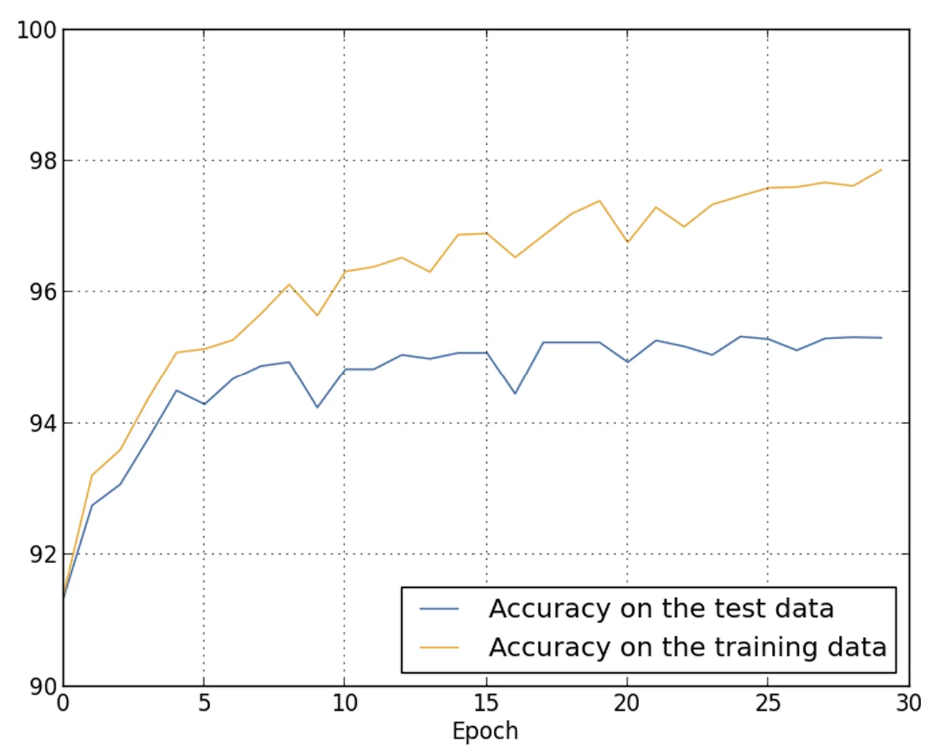
Note

As the plot illustrates, the accuracy on the training data and the accuracy on the test data remain much closer to each other compared to the case where training was performed on only $1, 000$ images. Specifically, the maximum accuracy on the training data (97.86%) exceeds that on the test data (95.33%) by only 2.53 percentage points, compared to the 17.73% gap observed earlier.
Overfitting is still present, but it is drastically reduced: the network generalizes significantly better.

Data Are the Essential Ingredient in Deep Learning

In general, increasing the size of the training set is one of the most effective strategies for mitigating overfitting.
With sufficient data, even very complex networks struggle to overfit.
However, acquiring large volumes of training data can be costly or difficult, limiting the practical applicability of this solution.

Appendix: overfitting.py

Note

This script depends on two additional modules:

network2 (defines the Network class and training functions)

mnist_loader.py (handles loading the MNIST dataset).

To make the script work, place overfitting.py, network2 , and mnist_loader.py in the same folder.

If the files are stored in different locations, the import paths inside overfitting.py must be adjusted accordingly.

"""
overfitting.py
~~~~~~~~~~~~~~
 
Plot graphs to illustrate the problem of overfitting.
 
Code adapted from Michael Nielsen's
"Neural Networks and Deep Learning"
https://github.com/mnielsen/neural-networks-and-deep-learning
 
MIT License (c) 2012-2018 Michael Nielsen
See https://opensource.org/licenses/MIT for details.
"""
 
# Standard library
import json
import random
import sys
 
# Nielsen's custom libraries
import mnist_loader
import network2
 
# Third-party libraries
import matplotlib.pyplot as plt
import numpy as np
 
 
def main(filename, num_epochs,
         training_cost_xmin=200, 
         test_accuracy_xmin=200, 
         test_cost_xmin=0, 
         training_accuracy_xmin=0,
         training_set_size=1000, 
         lmbda=0.0):
    """``filename`` is the name of the file where the results will be
    stored.  ``num_epochs`` is the number of epochs to train for.
    ``training_set_size`` is the number of images to train on.
    ``lmbda`` is the regularization parameter.  The other parameters
    set the epochs at which to start plotting on the x axis.
    """
    run_network(filename, num_epochs, training_set_size, lmbda)
    make_plots(filename, num_epochs, 
               training_cost_xmin,
               test_accuracy_xmin,
               test_cost_xmin, 
               training_accuracy_xmin,
               training_set_size)
                       
def run_network(filename, num_epochs, training_set_size=1000, lmbda=0.0):
    """Train the network for ``num_epochs`` on ``training_set_size``
    images, and store the results in ``filename``.  Those results can
    later be used by ``make_plots``.  Note that the results are stored
    to disk in large part because it's convenient not to have to
    ``run_network`` each time we want to make a plot (it's slow).
 
    """
    # Make results more easily reproducible
    random.seed(12345678)
    np.random.seed(12345678)
    training_data, validation_data, test_data = mnist_loader.load_data_wrapper()
    net = network2.Network([784, 30, 10], cost=network2.CrossEntropyCost())
    net.large_weight_initializer()
    test_cost, test_accuracy, training_cost, training_accuracy \
        = net.SGD(training_data[:training_set_size], num_epochs, 10, 0.5,
                  evaluation_data=test_data, lmbda = lmbda,
                  monitor_evaluation_cost=True, 
                  monitor_evaluation_accuracy=True, 
                  monitor_training_cost=True, 
                  monitor_training_accuracy=True)
    f = open(filename, "w")
    json.dump([test_cost, test_accuracy, training_cost, training_accuracy], f)
    f.close()
 
def make_plots(filename, num_epochs, 
               training_cost_xmin=200, 
               test_accuracy_xmin=200, 
               test_cost_xmin=0, 
               training_accuracy_xmin=0,
               training_set_size=1000):
    """Load the results from ``filename``, and generate the corresponding
    plots. """
    f = open(filename, "r")
    test_cost, test_accuracy, training_cost, training_accuracy \
        = json.load(f)
    f.close()
    plot_training_cost(training_cost, num_epochs, training_cost_xmin)
    plot_test_accuracy(test_accuracy, num_epochs, test_accuracy_xmin)
    plot_test_cost(test_cost, num_epochs, test_cost_xmin)
    plot_training_accuracy(training_accuracy, num_epochs, 
                           training_accuracy_xmin, training_set_size)
    plot_overlay(test_accuracy, training_accuracy, num_epochs,
                 min(test_accuracy_xmin, training_accuracy_xmin),
                 training_set_size)
 
def plot_training_cost(training_cost, num_epochs, training_cost_xmin):
    fig = plt.figure()
    ax = fig.add_subplot(111)
    ax.plot(np.arange(training_cost_xmin, num_epochs), 
            training_cost[training_cost_xmin:num_epochs],
            color='#2A6EA6')
    ax.set_xlim([training_cost_xmin, num_epochs])
    ax.grid(True)
    ax.set_xlabel('Epoch')
    ax.set_title('Cost on the training data')
    plt.show()
 
def plot_test_accuracy(test_accuracy, num_epochs, test_accuracy_xmin):
    fig = plt.figure()
    ax = fig.add_subplot(111)
    ax.plot(np.arange(test_accuracy_xmin, num_epochs), 
            [accuracy/100.0 
             for accuracy in test_accuracy[test_accuracy_xmin:num_epochs]],
            color='#2A6EA6')
    ax.set_xlim([test_accuracy_xmin, num_epochs])
    ax.grid(True)
    ax.set_xlabel('Epoch')
    ax.set_title('Accuracy (%) on the test data')
    plt.show()
 
def plot_test_cost(test_cost, num_epochs, test_cost_xmin):
    fig = plt.figure()
    ax = fig.add_subplot(111)
    ax.plot(np.arange(test_cost_xmin, num_epochs), 
            test_cost[test_cost_xmin:num_epochs],
            color='#2A6EA6')
    ax.set_xlim([test_cost_xmin, num_epochs])
    ax.grid(True)
    ax.set_xlabel('Epoch')
    ax.set_title('Cost on the test data')
    plt.show()
 
def plot_training_accuracy(training_accuracy, num_epochs, 
                           training_accuracy_xmin, training_set_size):
    fig = plt.figure()
    ax = fig.add_subplot(111)
    ax.plot(np.arange(training_accuracy_xmin, num_epochs), 
            [accuracy*100.0/training_set_size 
             for accuracy in training_accuracy[training_accuracy_xmin:num_epochs]],
            color='#2A6EA6')
    ax.set_xlim([training_accuracy_xmin, num_epochs])
    ax.grid(True)
    ax.set_xlabel('Epoch')
    ax.set_title('Accuracy (%) on the training data')
    plt.show()
 
def plot_overlay(test_accuracy, training_accuracy, num_epochs, xmin,
                 training_set_size):
    fig = plt.figure()
    ax = fig.add_subplot(111)
    ax.plot(np.arange(xmin, num_epochs), 
            [accuracy/100.0 for accuracy in test_accuracy], 
            color='#2A6EA6',
            label="Accuracy on the test data")
    ax.plot(np.arange(xmin, num_epochs), 
            [accuracy*100.0/training_set_size 
             for accuracy in training_accuracy], 
            color='#FFA933',
            label="Accuracy on the training data")
    ax.grid(True)
    ax.set_xlim([xmin, num_epochs])
    ax.set_xlabel('Epoch')
    ax.set_ylim([90, 100])
    plt.legend(loc="lower right")
    plt.show()
 
if __name__ == "__main__":
    filename = input("Enter a file name: ")
    num_epochs = int(input(
        "Enter the number of epochs to run for: "))
    training_cost_xmin = int(input(
        "training_cost_xmin (suggest 200): "))
    test_accuracy_xmin = int(input(
        "test_accuracy_xmin (suggest 200): "))
    test_cost_xmin = int(input(
        "test_cost_xmin (suggest 0): "))
    training_accuracy_xmin = int(input(
        "training_accuracy_xmin (suggest 0): "))
    training_set_size = int(input(
        "Training set size (suggest 1000): "))
    lmbda = float(input(
        "Enter the regularization parameter, lambda (suggest: 5.0): "))
    main(filename, num_epochs, training_cost_xmin, 
         test_accuracy_xmin, test_cost_xmin, training_accuracy_xmin,
         training_set_size, lmbda)

Deep Learning

Explorer

Overfitting on MNIST

Experiment 1 – Reduced Dataset

Results

Training Loss and Test Accuracy

Training and Test Loss

Training and Test Accuracy

Overfitting mitigation

Early Stopping (with Test Set)

Using a Validation set

Experiment 2 – Full Dataset

Results

Appendix: overfitting.py

Graph View

Table of Contents

Backlinks