Data Augmentation

Intro

Data is the fundamental ingredient of Deep Learning

The current success of Deep Learning is largely determined by the quantity and quality of available data. Among the strategies to mitigate overfitting catalogued in the introduction of this section, “use more data” is the most effective, and often the one with the largest absolute impact on test performance.

Using more data is the cleanest cure for overfitting. In practice, however, the amount of available data is almost always limited by collection costs, annotation costs, or privacy constraints. Data augmentation is the systematic answer to this limitation: artificially generate new training examples by applying transformations to existing ones, then feed the augmented examples to the network at training time alongside the originals.

Augmentation is always domain-specific

Different data modalities admit different transformations. The notion of “a valid transformation” depends on what aspects of the input are semantically relevant for the task and what aspects are not.

For images, classical image-processing techniques double as augmentation primitives:

contrast enhancement,

histogram equalization,

denoising,

noise injection,

geometric transformations (rotations, flips, crops, scaling, translation, shearing),

colour-space perturbations (brightness, saturation, hue jitter),

cutout / masking of random patches.

For text (NLP), augmentation is typically done via synonym replacement, random word deletion, back-translation (translate to a second language and back), or paraphrasing with a language model.

For audio, common augmentations include time-stretching, pitch-shifting, additive background noise, and SpecAugment-style masking of frequency or time bands in the spectrogram.

For tabular data, augmentation is harder: random perturbations rarely preserve semantic validity, and the most useful techniques are model-based (SMOTE, generative-model resampling).

More heterogeneity is good, up to a point

The greater the heterogeneity introduced by augmentation, the better the network’s chances of generalizing to data it has not seen, as long as the transformations remain semantically valid. Heterogeneity that destroys the meaning of the data corrupts the supervision signal and turns the regularizer into a source of noise.

Inappropriate augmentation backfires

When augmentation is applied without care, it can introduce semantic distortions that harm rather than help training. The remainder of this note catalogues the three most common failure modes (not-representative, too-much, biased augmentation) and the rules of thumb that mitigate each one.

The golden rule: semantic coherence

The single most important principle is the following.

The golden rule

An augmentation transformation must not change the meaning of the data. A transformed image must remain a plausible, correctly-labelled example of its class. A paraphrased sentence must still express the same sentiment. A pitch-shifted utterance must still be the same phoneme.

Any augmentation that breaks this invariant is not extending the training set; it is corrupting it.

When augmentation actively hurts

If a transformation introduces unrealistic distortions, or alters the perceived label, it stops being useful and becomes an obstacle. A textbook example is rotating brain MRI scans: clinical MRIs are already registered to a standard anatomical reference frame, so applying a random rotation does not produce a realistic new patient, it produces an off-axis scan that no real protocol would ever output. The model is forced to learn that off-axis scans are also instances of the disease, which is false, and the resulting predictions degrade.

A worked example: the MNIST “6 vs 9” trap

The figure below illustrates a clean case where augmentation creates synthetic variants of a hand-written digit from MNIST.

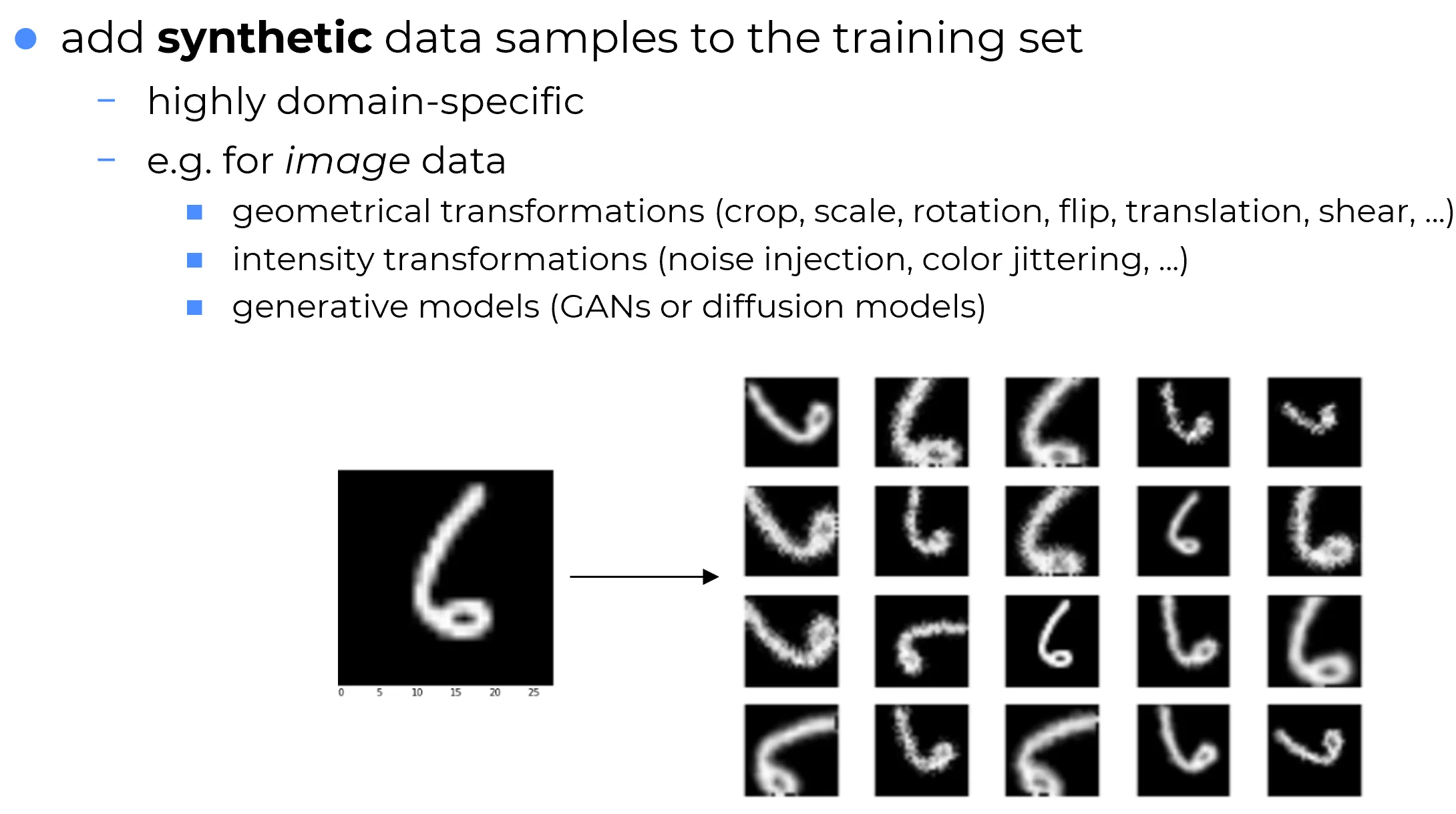
For the digit “6”, an extreme rotation (e.g., $180°$ ) produces an image that visually resembles a “9”, while the label remains “6” because the augmentation pipeline preserves the original target. The model then receives a contradictory training signal: the visual representation has changed dramatically, but the supervision says “still a 6”.

The consequences are unfailingly bad.

Two failure scenarios

Poor learning during training. The network fails to identify coherent patterns because of the noise introduced by semantically invalid transformations. The training loss does not show the typical smooth decay; instead it plateaus high or oscillates, signalling that the model is not learning a generalizable mapping.

Good training, terrible inference. A subtler and more dangerous outcome: the model memorizes the augmentation artifacts (the specific rotation angles, the specific blur patterns) rather than learning the discriminative features. Training loss decreases beautifully, but test accuracy collapses on real, un-augmented data. The model has effectively memorized the augmentation technique used, not the underlying digits.

The remedy for the MNIST example

Define semantically safe transformation ranges specific to the task. For hand-written digits, rotations should be limited to roughly $\pm 45°$ (a rotation of $\pm 30°$ is more conservative and almost always safe). Beyond that range, the digit’s identity is no longer preserved, and augmentation crosses from regularization into label corruption.

Without this safeguard, augmentation becomes a memorization mechanism

Augmentation that violates the golden rule does not just fail to help; it actively encourages the network to memorize artifacts, defeating its own purpose (which was, originally, to mitigate exactly this kind of memorization).

Three common failure modes

The three failure modes below recur across almost every domain. Each one has a short empirical description, the mechanism by which it harms the model, and a rule-of-thumb remedy.

Not representative augmentation

Symptom

The augmented examples do not reflect the distribution the model will actually face at inference. Concretely, transformations are applied that produce inputs the test set will never contain.

Example. In an OCR task on printed or hand-written text, rotations larger than $45°$ produce inputs that no real document would ever contain (documents are scanned approximately upright). The model is exposed to inputs that look nothing like its eventual operating regime.

The consequence depends on how extreme the mis-representation is. In the mild case, the model wastes capacity on irrelevant input regions and converges more slowly. In the severe case, the model fails to learn at all, because the apparent distribution becomes so heterogeneous that no consistent decision rule fits all the training examples. The training loss stays high and unstable, signalling that the model is misled by the extreme data heterogeneity.

Solution: start safe, expand gradually

Begin with simple, semantically sound augmentations that are demonstrably within the operating distribution, and add more aggressive transformations only as needed. Monitor the validation accuracy as new augmentations are introduced; if a new transformation degrades it, that transformation is producing inputs the model is not expected to handle and should be removed or scaled back.

Too much augmentation

Symptom

The training distribution becomes overwhelmingly synthetic. If the training set contains, say, $1%$ real examples and $99%$ augmented examples, the model’s learned distribution is essentially the distribution of the augmentation technique itself, not of the underlying real data.

The network may then fit the synthetic distribution very well and fail to generalize to real data at test time, because real data lives in a slightly different distribution that was crowded out by the augmented one.

The mechanism is the same as the MNIST trap above, but operating at the population level rather than at the per-example level: it is not any single transformation that breaks the labels, it is the ratio of synthetic to real that pushes the model into memorizing the synthesis pipeline. Even augmentations that individually preserve semantics can, when applied in overwhelming proportion, distort the empirical distribution enough that the model learns the augmentation rather than the task.

Solution: start with a 1:1 ratio, increase gradually

A reasonable default is to begin with roughly one augmented example per real example (a $1 : 1$ ratio), then increase the augmentation rate progressively while watching the validation accuracy. The right ratio is highly domain-dependent:

in biomedical imaging, where real examples are scarce and augmentations are well-validated, ratios like $1 : 10$ are routine;

in natural images with abundant data, ratios closer to $1 : 1$ or even less aggressive augmentation are common;

in NLP, where text-level augmentations are themselves noisy, low ratios ( $1 : 0.5$ , i.e.\ augmentation on only half of the training set) are often preferred.

No single ratio is universally correct. The principle is to let the validation set decide.

Biased augmentation

Symptom (subtle and dangerous)

Biased augmentation occurs when augmentations are applied unevenly across the classes. For example, in a binary cat/dog classifier, the cats are rotated and the dogs are not; or the cat images receive brightness jitter and the dog images receive crop augmentation.

Neural networks are excellent memorizers. If a transformation is applied systematically to one class and not to another, the network can reverse-engineer the augmentation policy and use the augmentation artifacts themselves to discriminate samples from different classes, rather than the actual discriminative features (the shape of the snout, the texture of the fur, and so on).

The pathology is insidious because it produces good training accuracy and good validation accuracy if the validation set is augmented in the same biased way. It only surfaces on real, un-augmented test data, by which point the production pipeline has already learned an artificial decision rule.

This pattern belongs to a broader family of problems in which augmentation introduces systematic differences across classes: any such systematic difference can be picked up by the network as a discriminative cue, even when it has no real-world meaning.

Solution: just do not do it

The augmentation pipeline must be class-agnostic. The same set of transformations, with the same probabilities and the same parameter ranges, must be applied uniformly across all classes. If a particular augmentation makes sense only for some classes (a rare but possible case), the imbalance must be documented and its effect on the model audited explicitly. Outside of these audited exceptions, the rule is simple: never apply different augmentations to different classes.

Modern automated augmentation

A practical observation about augmentation design: manually choosing which transformations to apply, with which probabilities, and within which ranges is tedious and error-prone. Several lines of work have automated this choice.

Three notable approaches

AutoAugment (Cubuk et al., 2019) treats augmentation policy selection as a reinforcement-learning problem: a controller proposes augmentation policies, child networks are trained briefly on each, and the controller is rewarded for policies that produce high validation accuracy. Expensive but produces strong policies for ImageNet, CIFAR, and SVHN.

RandAugment (Cubuk et al., 2020) drastically simplifies the search: at every batch, $N$ augmentations are sampled uniformly from a fixed list, each applied with magnitude $M$ . The hyperparameters $(N, M)$ are tuned by a simple grid search. Almost as effective as AutoAugment at a fraction of the search cost.

TrivialAugment (Müller and Hutter, 2021) takes the simplification further: at every example, one augmentation is sampled uniformly from a list, with magnitude sampled uniformly from a range. No tuning at all. Competitive with both AutoAugment and RandAugment despite having no learnable hyperparameters.

The empirical trajectory here is informative: increasingly simple automated policies have caught up with increasingly complex ones, suggesting that the precise composition of an augmentation policy matters less than the broad principles described in this note. Random sampling from a sensible list of class-agnostic, semantically-valid transformations is usually within a percentage point of the most elaborate hand-tuned schedule.

Strong augmentations: Mixup and CutMix

Two augmentation techniques that have become standard in modern image classification go beyond the “single-image transformation” paradigm by mixing pairs of training examples.

Mixup and CutMix

Mixup (Zhang et al., 2018) creates a new training example by taking a convex combination of two real examples and their labels:
$\tilde{x} = λ x_{i} + (1 - λ) x_{j}, \tilde{y} = λ y_{i} + (1 - λ) y_{j},$
where $λ \sim Beta (α, α)$ for a small $α$ (typically $0.1$ to $0.4$ ). The coefficients $λ$ and $1 - λ$ are non-negative and sum to $1$ , so $(\tilde{x}, \tilde{y})$ sits on the line segment between the two real examples in input space and on the corresponding line segment between their one-hot labels. The mixed image looks like a translucent overlay of two scenes; the mixed label is a soft mixture of the two class probabilities.

CutMix (Yun et al., 2019) replaces a rectangular patch of one image with a patch from another, and mixes the labels in proportion to the patch area. The result is more spatially realistic than Mixup and tends to outperform it on object-classification benchmarks.

Both techniques act as strong regularizers: they prevent the network from being too confident on any single training example, and they push it toward smoother decision boundaries between classes. The mechanism is closely related in spirit to the Dropout perturbation: both inject training-time noise that the model must learn to be robust against.

Tools and libraries

Implementing the transformations of this note from scratch is rarely the right move: every modern deep-learning ecosystem ships at least one mature, performant augmentation library that handles the common image, text and audio transformations correctly, efficiently, and with sensible defaults.

A few mainstream libraries

torchvision.transforms (PyTorch). The built-in option: composable, well-integrated with Dataset and DataLoader, includes both the classical primitives (rotation, crop, jitter) and the modern automated policies (RandAugment, TrivialAugmentWide, AutoAugment).

Albumentations. The de-facto standard for high-throughput image augmentation in modern computer-vision pipelines: faster than torchvision for several operations, with broad support for object detection, segmentation, and keypoint tasks (which require the augmentation to transform images and their annotations consistently). The library covers most of the techniques in this note and many additional ones; a dedicated note may be added in the future.

nlpaug for text augmentation, audiomentations for audio.

The choice of library is largely a matter of ecosystem and ergonomics; the principles in this note (semantic coherence, class-agnostic application, conservative magnitudes, validation-based tuning) apply regardless of the library used.