Cell state

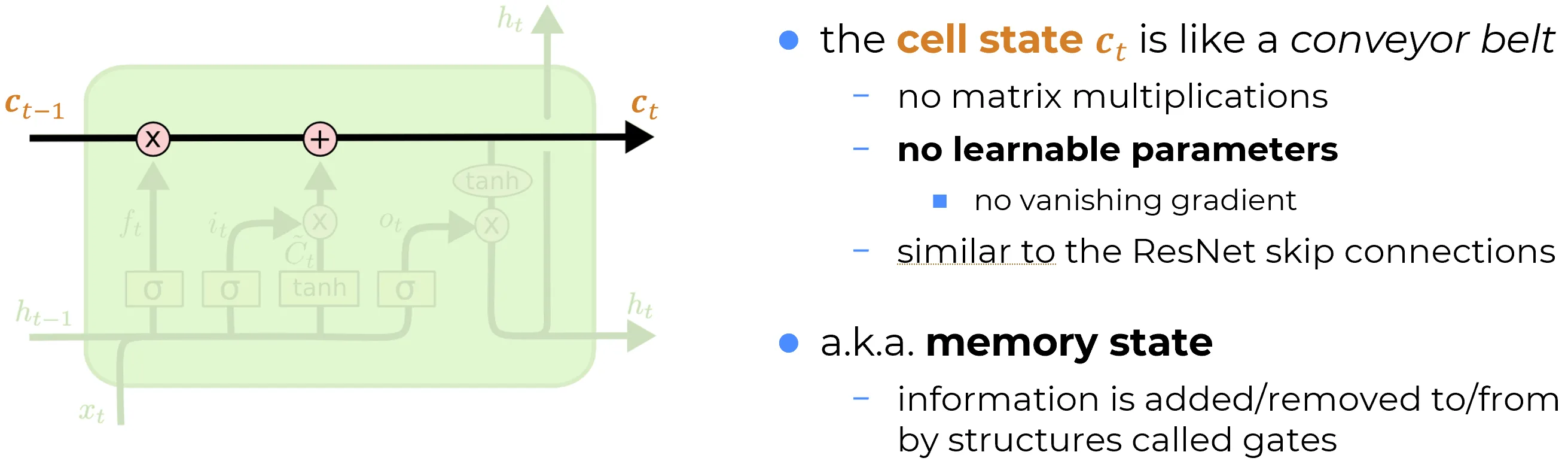
The black line at the top of the diagram is the cell state ${\mathbf{c}}_t$. It is the single most important object in the LSTM, because it is the place where the architectural fix anticipated in Vanilla RNNs limitations is implemented. Everything else in the cell exists to regulate what happens on this line.

What the line actually contains

Along the cell-state path, between ${\mathbf{c}}_{t-1}$ on the left and ${\mathbf{c}}_t$ on the right, only two operations are performed:

• an element-wise multiplication by the forget gate ${\mathbf{f}}_t\in (0,1{)}^{n_{\text{neurons}}}$;
• an element-wise addition of the gated candidate ${\mathbf{i}}_t\odot {\tilde{\mathbf{c}}}_t$.

The resulting update is

$${\mathbf{c}}_t={\mathbf{f}}_t\odot {\mathbf{c}}_{t-1}+{\mathbf{i}}_t\odot {\tilde{\mathbf{c}}}_t.$$

The forget gate ${\mathbf{f}}_t$, the input gate ${\mathbf{i}}_t$ and the candidate ${\tilde{\mathbf{c}}}_t$ are produced by separate small networks, off to the side; they connect to the cell-state line only through the two $\odot$ junctions. The line itself never crosses a weight matrix and never goes through a non-linearity.

Dimensions used in this note

symbol	role	shape
${\mathbf{c}}_{t-1},{\mathbf{c}}_t$	cell state	$n_{\text{neurons}}$
${\mathbf{f}}_t,{\mathbf{i}}_t$	gates (defined elsewhere)	$n_{\text{neurons}}$
${\tilde{\mathbf{c}}}_t$	candidate update (defined in [[input-gate	Input gate]])

All element-wise products $\odot$ on this line act on operands of identical shape $n_{\text{neurons}}$, so no broadcasting is involved.

No parameters on the carry path

Read the diagram once more with this in mind: the route from ${\mathbf{c}}_{t-1}$ to ${\mathbf{c}}_t$ contains zero learnable weights and zero saturating activations. The gates inject parameters into the path through pointwise products, but the path itself is purely arithmetic.

This is what makes the cell state a skip connection along time. Information and gradient can travel along it for hundreds of steps without being squeezed through a matrix product or a tanh; the only thing that can attenuate them is the forget gate, and that attenuation is learned, not imposed.

Why this is the cure for vanishing gradients

The recurrent Jacobian along the cell-state line is, by direct differentiation of the update equation,

$$\frac{\partial {\mathbf{c}}_t}{\partial {\mathbf{c}}_{t-1}}=\mathrm{diag}({\mathbf{f}}_t).$$

Coordinate independence: "no cross-coordinate mixing"

The Jacobian above is diagonal, not just small or bounded. The reason is a structural property of the operations on the cell-state line: the element-wise product $\odot$, the pointwise sigmoid and the pointwise tanh all act one coordinate at a time,

$$(\mathbf{a}\odot \mathbf{b}{)}^{(j)}=a^{(j)}{b}^{(j)},\sigma (\mathbf{z}{)}^{(j)}=\sigma (z^{(j)}),\tanh (\mathbf{z}{)}^{(j)}=\tanh (z^{(j)}),$$

never producing terms in which an output coordinate $j$ depends on an input coordinate $k\ne j$. This is the property referred to throughout the LSTM notes as “no cross-coordinate mixing”, or equivalently coordinate independence of the update.

Inside the LSTM, cross-coordinate mixing happens only in the four affine maps ${\mathbf{W}}_{x\bullet }{\mathbf{x}}_t+{\mathbf{W}}_{h\bullet }{\mathbf{h}}_{t-1}$ that produce the gates and the candidate. The cell-state line itself, between ${\mathbf{c}}_{t-1}$ and ${\mathbf{c}}_t$, is by construction free of any such mixing, and that is why its Jacobian is diagonal at every step. The derivation below makes this concrete.

Derivation, coordinate by coordinate

Writing the cell state update component by component, the $j$-th coordinate of ${\mathbf{c}}_t$ is

$$c_t^{(j)}=({\mathbf{f}}_t\odot {\mathbf{c}}_{t-1}{)}^{(j)}+({\mathbf{i}}_t\odot {\tilde{\mathbf{c}}}_t{)}^{(j)}=f_t^{(j)}{c}_{t-1}^{(j)}+i_t^{(j)}{\tilde{c}}_t^{(j)}.$$

Two facts make this expression easy to differentiate with respect to ${\mathbf{c}}_{t-1}$:

• Coordinate independence of $\odot$ (see the callout above): $c_t^{(j)}$ depends on $c_{t-1}^{(k)}$ only when $k=j$.
• The gates ${\mathbf{f}}_t$, ${\mathbf{i}}_t$ and the candidate ${\tilde{\mathbf{c}}}_t$ are functions of $({\mathbf{x}}_t,{\mathbf{h}}_{t-1})$, not of ${\mathbf{c}}_{t-1}$, so they are constants under this partial derivative.

Both facts together give

$$\frac{\partial c_t^{(j)}}{\partial c_{t-1}^{(k)}}=f_t^{(j)}{\delta }_{jk},$$

where ${\delta }_{jk}$ is the Kronecker delta. Stacked into a matrix, this is the diagonal matrix with ${\mathbf{f}}_t$ on the diagonal:

$$\frac{\partial {\mathbf{c}}_t}{\partial {\mathbf{c}}_{t-1}}=\mathrm{diag}({\mathbf{f}}_t).$$

The implication of coordinate independence is that each slot of the cell state evolves as an independent scalar register, a point developed in Input gate.

Compare this with the vanilla RNN Jacobian derived in BPTT Problems,

$$\frac{\partial {\mathbf{h}}_t}{\partial {\mathbf{h}}_{t-1}}=\mathrm{diag}({\varphi }_h^{\prime }({\mathbf{a}}_t)){\mathbf{W}}_{hh},$$

and the structural difference becomes visible at a glance. The vanilla Jacobian is a dense matrix scaled by the slope of $\tanh$: its spectral norm depends on ${\mathbf{W}}_{hh}$, and the product across time either decays or blows up geometrically. The LSTM Jacobian is diagonal and bounded in $(0,1)$ per coordinate: across $k$ steps the product is

$$\prod _{s=t-k+1}^t\frac{\partial {\mathbf{c}}_s}{\partial {\mathbf{c}}_{s-1}}=\prod _{s=t-k+1}^t\mathrm{diag}({\mathbf{f}}_s)=\mathrm{diag}\left(\prod _{s=t-k+1}^t{\mathbf{f}}_s\right),$$

still diagonal, still bounded coordinate by coordinate. Setting ${\mathbf{f}}_s\approx 1$ along a direction keeps the product close to the identity for arbitrarily many steps; the gradient survives.

Why the product of diagonal matrices is diagonal

For two diagonal matrices $\mathrm{diag}(\mathbf{a})$ and $\mathrm{diag}(\mathbf{b})$ of the same size, ordinary matrix multiplication gives

$$(\mathrm{diag}(\mathbf{a})\mathrm{diag}(\mathbf{b}){)}_{jk}=\sum _{\ell }{a}_j{\delta }_{j\ell }\cdot b_{\ell }{\delta }_{\ell k}=a_j{b}_j{\delta }_{jk}.$$

So the product is again diagonal, and its $j$-th diagonal entry is the product of the $j$-th entries of $\mathbf{a}$ and $\mathbf{b}$. Equivalently:

$$\mathrm{diag}(\mathbf{a})\mathrm{diag}(\mathbf{b})=\mathrm{diag}(\mathbf{a}\odot \mathbf{b}).$$

Iterating, the product of $k$ diagonal matrices is the diagonal matrix of element-wise products:

$$\prod _{s=t-k+1}^t\mathrm{diag}({\mathbf{f}}_s)=\mathrm{diag}\left(\underset{s=t-k+1}{\overset{t}{⨀}}{\mathbf{f}}_s\right).$$

This is what makes the gradient analysis along the cell-state line a per-coordinate statement: there is no mixing across coordinates as steps accumulate.

The full backward-pass analysis is carried out in Gradient in LSTM.

The constant error carousel

In the original Hochreiter–Schmidhuber paper, the configuration ${\mathbf{f}}_s=1$, ${\mathbf{i}}_s=0$ is called the Constant Error Carousel (CEC): the cell state evolves as ${\mathbf{c}}_t={\mathbf{c}}_{t-1}$ and the error signal travels along the carousel without any change in magnitude. The 1997 paper actually proposed the cell with this CEC as the centerpiece; the forget gate was added later by Gers, Schmidhuber and Cummins in 2000 so that the carousel could also learn to stop.

The cell state is a leaky integrator

With the gates held fixed for a moment, $f_t^{(j)}=f^{(j)}$ and $i_t^{(j)}=i^{(j)}$, substitute the scalar recursion $c_t^{(j)}=f^{(j)}{c}_{t-1}^{(j)}+i^{(j)}{\tilde{c}}_t^{(j)}$ into itself repeatedly:

$$c_t^{(j)}=i^{(j)}{\tilde{c}}_t^{(j)}+f^{(j)}(i^{(j)}{\tilde{c}}_{t-1}^{(j)}+f^{(j)}{c}_{t-2}^{(j)})=\cdots =\sum _{k=0}^{t-1}(f^{(j)}{)}^k{i}^{(j)}{\tilde{c}}_{t-k}^{(j)}+(f^{(j)}{)}^t{c}_0^{(j)}.$$

Each step pushes the running memory through one more factor of $f^{(j)}$, so the input from $k$ steps ago survives with weight $(f^{(j)}{)}^k$: each slot is an exponentially weighted moving average of its past inputs. This is the same exponential average that drives the velocity in momentum and the moments in Adam. The weights sum to ${\sum }_{k\ge 0}(f^{(j)}{)}^k=1/(1-f^{(j)})$ for $f^{(j)}<1$, so the slot’s memory horizon is about $1/(1-f^{(j)})$ steps: a decay of $0.99$ remembers roughly a hundred steps, $0.999$ a thousand, and the constant error carousel is the limit $f^{(j)}=1$ with infinite horizon.

The one thing the LSTM adds over a fixed moving average is that $f_t^{(j)}$ is recomputed at every step from $({\mathbf{x}}_t,{\mathbf{h}}_{t-1})$. The decay is data-dependent and per-coordinate, so the cell can lengthen or shorten the memory of each slot in response to what it is currently reading.

The architectural pattern this exemplifies

The cell-state line is the historical ancestor of a pattern that recurs throughout modern deep learning: isolate an identity path through the model, and let learned modules perturb the state living on that path, never carry it themselves.

• In a ResNet block, the input $\mathbf{x}$ travels through the identity shortcut while a small residual function $\mathcal{F}(\mathbf{x})$ is added to it. The Jacobian of $\mathbf{x}+\mathcal{F}(\mathbf{x})$ with respect to $\mathbf{x}$ is $\mathbf{I}+\partial \mathcal{F}/\partial \mathbf{x}$, so gradient flows through $\mathbf{I}$ unimpeded across depth.
• In a Transformer block, the residual stream plays exactly the same role across layers, with attention and MLP sublayers contributing additive updates.
• In the LSTM cell, the cell state ${\mathbf{c}}_t$ is the residual stream across time, with the gated update ${\mathbf{i}}_t\odot {\tilde{\mathbf{c}}}_t$ playing the role of $\mathcal{F}$ and the forget gate adding a learned per-coordinate decay.

The LSTM came first, in 1997, six years before residual connections were introduced in feedforward networks by He et al. (2015). Reading it as a temporal residual stream is the cleanest way to see why it works, and why the same idea later made very deep feedforward and Transformer architectures possible.

One difference worth naming

A vanilla residual connection has Jacobian exactly $\mathbf{I}$ on the shortcut: it never forgets. The LSTM’s Jacobian along the cell state is $\mathrm{diag}({\mathbf{f}}_t)$, which can decide to forget on a per-coordinate, per-step basis. The cell state is, in this sense, a learnable residual stream, slightly more expressive than a static identity shortcut. This added flexibility is also what makes the LSTM’s memory finite in practice: it can choose to clear itself.

That same data-dependent decay is the idea selective state-space models (Mamba, 2023) later reintroduced to rival attention on long sequences. Classical linear state-space models fix their recurrence coefficients, which parallelizes cleanly across time but cannot choose what to keep; making those coefficients input-dependent, exactly as the forget gate does, restores the selectivity. The LSTM had the mechanism in 1997, and the later work kept the input-dependent gating while changing only how it is computed, so that it parallelizes across the sequence.

The next three notes build the gates that act on this line one at a time, in the order in which they touch ${\mathbf{c}}_t$: the forget gate first, which scales ${\mathbf{c}}_{t-1}$; then the input gate together with the candidate ${\tilde{\mathbf{c}}}_t$, which add new content; and finally the output gate, which decides how much of the updated ${\mathbf{c}}_t$ to expose as the hidden state ${\mathbf{h}}_t$.