LSTM Layer overview

The architectural prescription from Vanilla RNNs limitations (additive memory plus a learned forget gate) is built here in full, one piece at a time, in the order in which information flows through the LSTM cell.

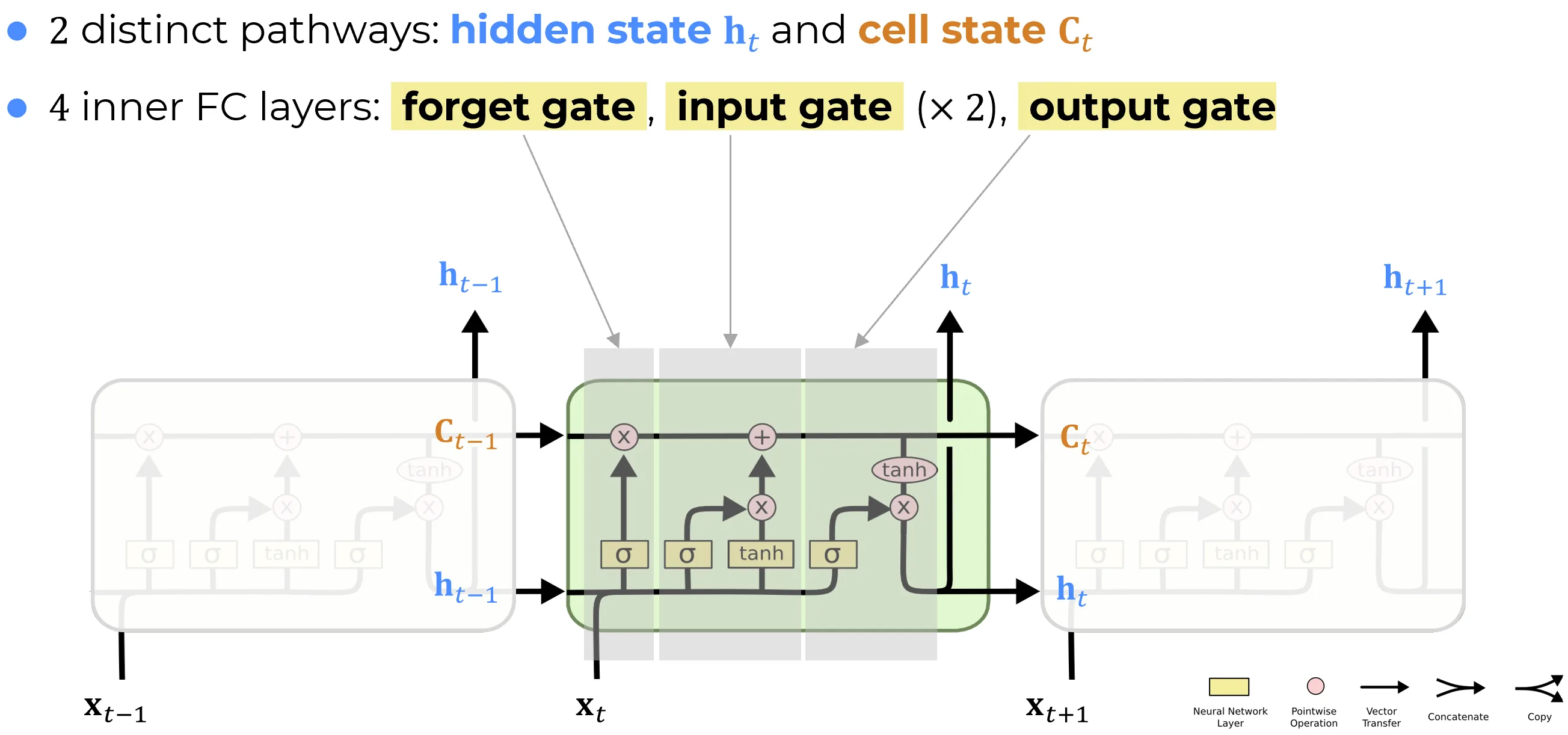
1. LSTM Layer overview: the two states (${\mathbf{c}}_t$, ${\mathbf{h}}_t$), the four inner FC layers, and the notation used throughout the subsection.
2. Cell state: the carry line ${\mathbf{c}}_{t-1}\to {\mathbf{c}}_t$ as a temporal skip connection, and the canonical definition of coordinate independence that makes its Jacobian diagonal.
3. Forget gate: the gating of ${\mathbf{c}}_{t-1}$ by ${\mathbf{f}}_t$, the choice of sigmoid, and the consequential forget-bias initialization.
4. Input gate: the candidate update ${\tilde{\mathbf{c}}}_t$ (with tanh) and the input mask ${\mathbf{i}}_t$ (with sigmoid), and why the what and how much of writing are split into two separate networks.
5. Output gate: the read-out ${\mathbf{h}}_t={\mathbf{o}}_t\odot \tanh ({\mathbf{c}}_t)$ and the separation between what the cell stores (${\mathbf{c}}_t$) and what it says (${\mathbf{h}}_t$).
6. Putting all together: the complete forward pass, the mini-batch vectorization, the master dimensions table, the broadcasting audit, the parameter count, and the fused-weight matrix used by modern frameworks.

The gradient analysis of the assembled cell is treated separately in Gradient in LSTM, one level up.

---

The diagnosis of Vanilla RNNs limitations ends with a single architectural prescription: take the recurrent matrix off the carry path and replace overwriting with additive update through a learned gate. The LSTM cell is what that prescription looks like when written out in full. This note fixes the notation and the high-level reading of the diagram above; the gate-by-gate derivation begins with the cell state.

Notation used in this section

Throughout the LSTM layer notes:

• lowercase bold denotes a vector for a single example (${\mathbf{x}}_t,{\mathbf{h}}_t,{\mathbf{c}}_t,{\mathbf{f}}_t,{\mathbf{i}}_t,{\mathbf{o}}_t,{\tilde{\mathbf{c}}}_t$);
• uppercase bold denotes the corresponding mini-batch matrix, with one column per example (${\mathbf{X}}_t,{\mathbf{H}}_t,{\mathbf{C}}_t,{\mathbf{F}}_t,{\mathbf{I}}_t,{\mathbf{O}}_t,{\tilde{\mathbf{C}}}_t$), or a learned weight matrix (${\mathbf{W}}_{x\bullet },{\mathbf{W}}_{h\bullet }$).

The diagrams in this section label the cell state with an uppercase symbol because they depict a single time step in isolation; the equations always follow the convention above.

The two sizes: $n_{\text{inputs}}$ and $n_{\text{neurons}}$

Two integers fix the shape of everything in this section.

• $n_{\text{inputs}}$ is the number of features in each input vector ${\mathbf{x}}_t$: the dimensionality of one element of the sequence, such as the embedding size of a token or the channel count of a frame. It is set by the data.
• $n_{\text{neurons}}$ is the number of units in one LSTM layer, and it is a design choice. A unit carries one coordinate of the cell state and one coordinate of the hidden state; it is the recurrent analogue of a single neuron in a fully connected layer. There are $n_{\text{neurons}}$ of them, so every vector the cell computes at a step, ${\mathbf{c}}_t,{\mathbf{h}}_t,{\mathbf{f}}_t,{\mathbf{i}}_t,{\mathbf{o}}_t,{\tilde{\mathbf{c}}}_t$, has one entry per unit and therefore lives in ${\mathbb{R}}^{n_{\text{neurons}}}$, while only the input ${\mathbf{x}}_t$ lives in ${\mathbb{R}}^{n_{\text{inputs}}}$.

The name $n_{\text{neurons}}$ is therefore deliberate. The $n_{\text{neurons}}$ units sit side by side and all read the same input pair $({\mathbf{x}}_t,{\mathbf{h}}_{t-1})$; the original Hochreiter and Schmidhuber paper calls one such unit an LSTM block. To process a sequence the layer is unrolled over the $T$ time steps, reusing the same units at each one. In PyTorch this number is the constructor argument hidden_size.

Two states, two roles

At every step $t=1,\dots ,T$ an LSTM cell receives $({\mathbf{x}}_t,{\mathbf{h}}_{t-1},{\mathbf{c}}_{t-1})$ and produces $({\mathbf{h}}_t,{\mathbf{c}}_t)$. Unlike a vanilla RNN, which carries a single hidden vector forward, an LSTM carries two:

• the cell state ${\mathbf{c}}_t\in {\mathbb{R}}^{n_{\text{neurons}}}$, the orange label, which is the long-term memory of the cell;
• the hidden state ${\mathbf{h}}_t\in {\mathbb{R}}^{n_{\text{neurons}}}$, the blue label, which is the cell’s externally visible output.

Both are passed to the next time step; only ${\mathbf{h}}_t$ is exposed to the rest of the network (and to any prediction head built on top of the layer).

Why two states and not one

The two paths are not redundant: they obey different constraints, and the LSTM works because those constraints are incompatible inside a single vector.

• ${\mathbf{c}}_t$ must live in an unconstrained, additive space so that gradient can flow back through it unchanged across long gaps. This is the highway that fixes the vanishing gradient. Its components are not bounded.
• ${\mathbf{h}}_t$ must be bounded and selective: it is fed back into the gate computations at the next step (through sigmoids and a tanh), and it is the signal that downstream layers consume. A bounded, task-focused output is what makes both the gating logic and the prediction head well-behaved.

Squeezing both jobs into a single hidden vector is exactly what a vanilla RNN attempts, and exactly why it cannot preserve information: the same coordinate would have to be at once a long-lived unbounded register and a short-lived bounded summary. Separating the two is the architectural move.

The four inner FC layers

The diagram contains four small fully connected layers, each one a familiar affine map followed by a pointwise nonlinearity. They are not four independent modules: each consumes the same input pair $({\mathbf{x}}_t,{\mathbf{h}}_{t-1})$ and produces a vector in ${\mathbb{R}}^{n_{\text{neurons}}}$.

• Forget gate ${\mathbf{f}}_t=\sigma (\cdot )\in (0,1{)}^{n_{\text{neurons}}}$. Decides, component by component, what fraction of ${\mathbf{c}}_{t-1}$ to keep. Detailed in Forget gate.
• Input gate ${\mathbf{i}}_t=\sigma (\cdot )\in (0,1{)}^{n_{\text{neurons}}}$. Decides, component by component, how much of the new candidate to write. Detailed in Input gate.
• Candidate update ${\tilde{\mathbf{c}}}_t=\tanh (\cdot )\in (-1,1{)}^{n_{\text{neurons}}}$. Proposes a signed content vector to add to memory. Also covered in Input gate.
• Output gate ${\mathbf{o}}_t=\sigma (\cdot )\in (0,1{)}^{n_{\text{neurons}}}$. Decides, component by component, what part of the freshly updated memory to expose as ${\mathbf{h}}_t$. Detailed in Output gate.

The cell state update, anticipated in the limitations note and derived properly in Cell state, is

$${\mathbf{c}}_t={\mathbf{f}}_t\odot {\mathbf{c}}_{t-1}+{\mathbf{i}}_t\odot {\tilde{\mathbf{c}}}_t,$$

and the hidden state is read out from it as

$${\mathbf{h}}_t={\mathbf{o}}_t\odot \tanh ({\mathbf{c}}_t).$$

Dimensions used in this note

symbol	role	shape
${\mathbf{x}}_t$	current input	$n_{\text{inputs}}$
${\mathbf{h}}_{t-1},{\mathbf{h}}_t$	hidden state	$n_{\text{neurons}}$
${\mathbf{c}}_{t-1},{\mathbf{c}}_t$	cell state	$n_{\text{neurons}}$
${\mathbf{f}}_t,{\mathbf{i}}_t,{\mathbf{o}}_t$	gates	$n_{\text{neurons}}$
${\tilde{\mathbf{c}}}_t$	candidate update	$n_{\text{neurons}}$
${\mathbf{W}}_{x\bullet }$	input-to-hidden weights, $\bullet \in \{f,i,c,o\}$	$n_{\text{neurons}}\times n_{\text{inputs}}$
${\mathbf{W}}_{h\bullet }$	hidden-to-hidden weights	$n_{\text{neurons}}\times n_{\text{neurons}}$
${\mathbf{b}}_{\bullet }$	bias	$n_{\text{neurons}}$

Three heads on a tape

Read the four maps as the three heads of a learned tape recorder operating on the memory ${\mathbf{c}}_t$:

• ${\mathbf{f}}_t$ is an erase head, selecting which entries of the tape to clear before writing.
• $({\mathbf{i}}_t,{\tilde{\mathbf{c}}}_t)$ together act as a write head: ${\tilde{\mathbf{c}}}_t$ is the content to write, ${\mathbf{i}}_t$ is the per-position write mask.
• ${\mathbf{o}}_t$ is a read head, selecting which entries of the tape to expose as ${\mathbf{h}}_t$.

This is not just a metaphor: it is exactly the decomposition that makes preservation a learned decision rather than a knife-edge of the recurrent spectrum. Erasure, writing, and reading are independent and gated at the per-coordinate level.

Shared input, separate transforms

All four maps share the same input $({\mathbf{x}}_t,{\mathbf{h}}_{t-1})$. The diagram makes this explicit: the blue line carrying ${\mathbf{h}}_{t-1}$ and the line carrying ${\mathbf{x}}_t$ both fan out into all four FC blocks. Each block, however, owns its own weight matrices and bias:

$$\begin{array}{rl}{\mathbf{f}}_t& =\sigma ({\mathbf{W}}_{xf}{\mathbf{x}}_t+{\mathbf{W}}_{hf}{\mathbf{h}}_{t-1}+{\mathbf{b}}_f),\\ {\mathbf{i}}_t& =\sigma ({\mathbf{W}}_{xi}{\mathbf{x}}_t+{\mathbf{W}}_{hi}{\mathbf{h}}_{t-1}+{\mathbf{b}}_i),\\ {\tilde{\mathbf{c}}}_t& =\tanh ({\mathbf{W}}_{xc}{\mathbf{x}}_t+{\mathbf{W}}_{hc}{\mathbf{h}}_{t-1}+{\mathbf{b}}_c),\\ {\mathbf{o}}_t& =\sigma ({\mathbf{W}}_{xo}{\mathbf{x}}_t+{\mathbf{W}}_{ho}{\mathbf{h}}_{t-1}+{\mathbf{b}}_o).\end{array}$$

The shared input is what gives the LSTM its coherence: at every step, all four decisions are conditioned on the same view of the world, namely the current input and the previous hidden summary. The cell does not separately gather “context for forgetting” and “context for writing”; it gathers context once, and routes it through four learned linear readouts.

The 4× parameter cost is not a bug

A vanilla RNN of width $n_{\text{neurons}}$ has one affine map of size $(n_{\text{inputs}}+n_{\text{neurons}})\times n_{\text{neurons}}$. An LSTM has four. The parameter count is therefore roughly $4\times$ larger at the same width.

This factor of four is the price of preservation. Three of the four maps exist exclusively to make the cell state behave as an unbiased additive register: one to erase, one to gate writes, one to gate reads. Only the candidate ${\tilde{\mathbf{c}}}_t$ plays the role of “what the vanilla RNN was already trying to compute”. Trading parameters for stable long-range gradient flow is the explicit bargain of the architecture, and it is what GRUs later try to renegotiate.

Unrolling and parameter sharing

The figure shows a single time step. As in the vanilla RNN, the cell is unrolled in time into as many copies as the sequence requires, and every copy shares the exact same parameters $\{{\mathbf{W}}_{x\bullet },{\mathbf{W}}_{h\bullet },{\mathbf{b}}_{\bullet }{\}}_{\bullet \in \{f,i,c,o\}}$. The initial states are conventionally fixed:

$${\mathbf{h}}_0=0,{\mathbf{c}}_0=0.$$

Training proceeds via Backpropagation Through Time on this unrolled graph, in any of its practical variants. The crucial property that motivated the whole construction, namely that gradient flows back through ${\mathbf{c}}_t$ with Jacobian $\mathrm{diag}({\mathbf{f}}_t)$ rather than through a product of recurrent matrices, is analyzed in Gradient in LSTM.

How to read the rest of this section

The remaining notes build the cell one piece at a time, in the order in which information flows through the diagram:

1. Cell state: the additive memory line ${\mathbf{c}}_{t-1}\to {\mathbf{c}}_t$ and its interpretation as a temporal skip connection.
2. Forget gate: the gating of ${\mathbf{c}}_{t-1}$ by ${\mathbf{f}}_t$.
3. Input gate: the candidate ${\tilde{\mathbf{c}}}_t$ and the input mask ${\mathbf{i}}_t$.
4. Output gate: the read-out ${\mathbf{h}}_t={\mathbf{o}}_t\odot \tanh ({\mathbf{c}}_t)$.
5. Putting all together: the complete forward pass and the mini-batch vectorization.